Project 2 - Rankine cycle Simulator
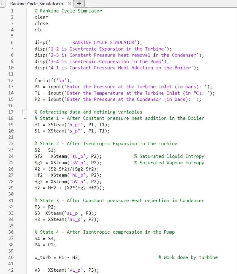
% Rankine Cycle Simulator
clear
close
clc

disp('        RANKINE CYCLE SIMULATOR');
disp('1-2 is Isentropic Expansion in the Turbine');
disp('2-3 is Constant Pressure heat removal in the Condenser');
disp('3-4 is Isentropic Compression in the Pump');
disp('4-1 is Constant Pressure Heat Addition in the Boiler');

fprintf('\n');
P1 = input('Enter the Pressure at the Turbine Inlet (in bars): ');
T1 = input('Enter the Temperature at the Turbine Inlet (in °C): ');
P2 = input('Enter the Pressure at the Condensor (in bars): ');

% Extracting data and defining variables
% State 1 - After Constant pressure heat addition in the Boiler
H1 = XSteam('h_pT', P1, T1);
S1 = XSteam('s_pT', P1, T1);

% State 2 - After Isentropic Expansion in the Turbine
S2 = S1;
Sf2 = XSteam('sL_p', P2);            % Saturated liquid Entropy
Sg2 = XSteam('sV_p', P2);            % Saturated Vapour Entropy
X2 = (S2-Sf2)/(Sg2-Sf2);             % Dryness Fraction
Hf2 = XSteam('hL_p', P2);
Hg2 = XSteam('hV_p', P2);
H2 = Hf2 + (X2*(Hg2-Hf2));

% State 3 - After Constant pressure Heat rejection in Condenser
P3 = P2;
S3= XSteam('sL_p', P3);
H3 = XSteam('hL_p', P3);

% State 4 - After Isentropic compression in the Pump
S4 = S3;
P4 = P1;

W_turb = H1 - H2;                             % Work done by turbine

V3 = XSteam('vL_p', P3);
W_pump = V3*(P4 - P3)*100;                    % Work done to run pump
H4 = H3 + W_pump;

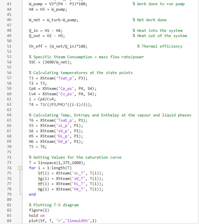
W_net = W_turb-W_pump;                        % Net Work done

Q_in = H1 - H4;                               % Heat into the system
Q_out = H2 - H3;                              % Heat out of the system

th_eff = (W_net/Q_in)*100;                      % Thermal efficiency

% Specific Steam Consumption = mass flow rate/power
SSC = (3600/W_net);

% Calculating temperatures at the state points
T3 = XSteam('Tsat_p', P3);
T2 = T3;
Cp4 = XSteam('Cp_ps', P4, S4);
Cv4 = XSteam('Cv_ps', P4, S4);
i = Cp4/Cv4;
T4 = T3/((P3/P4)^((i-1)/i));

% Calculating Temp, Entropy and Enthalpy at the vapour and liquid phases
T6 = XSteam('Tsat_p', P1);
S5 = XSteam('sL_p', P1);
S6 = XSteam('sV_p', P1);
H5 = XSteam('hL_p', P1);
H6 = XSteam('hV_p', P1);
T5 = T6;

% Getting Values for the saturation curve
T = linspace(1,375,1000);
for i = 1:length(T)
    Sf(i) = XSteam('sL_T', T(i));
    Sg(i) = XSteam('sV_T', T(i));
    Hf(i) = XSteam('hL_T', T(i));
    Hg(i) = XSteam('hV_T', T(i));
end

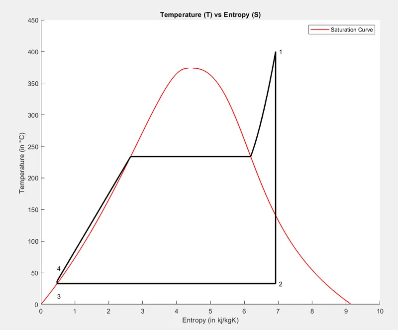
% Plotting T-S diagram
figure(1)
hold on
plot(Sf, T, 'r','linewidth',1)
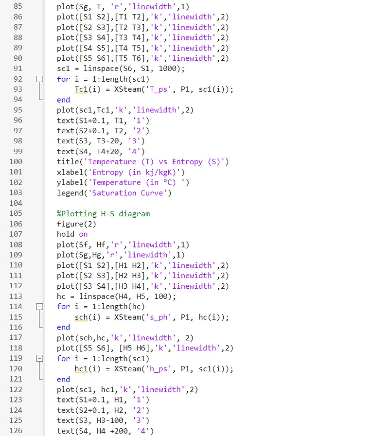
plot(Sg, T, 'r','linewidth',1)
plot([S1 S2],[T1 T2],'k','linewidth',2)
plot([S2 S3],[T2 T3],'k','linewidth',2)
plot([S3 S4],[T3 T4],'k','linewidth',2)
plot([S4 S5],[T4 T5],'k','linewidth',2)
plot([S5 S6],[T5 T6],'k','linewidth',2)
sc1 = linspace(S6, S1, 1000);
for i = 1:length(sc1)
    Tc1(i) = XSteam('T_ps', P1, sc1(i));
end
plot(sc1,Tc1,'k','linewidth',2)
text(S1+0.1, T1, '1')
text(S2+0.1, T2, '2')
text(S3, T3-20, '3')
text(S4, T4+20, '4')
title('Temperature (T) vs Entropy (S)')
xlabel('Entropy (in kj/kgK)')
ylabel('Temperature (in °C) ')
legend('Saturation Curve')

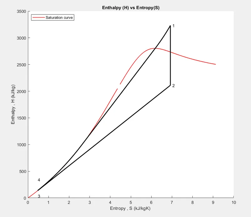
%Plotting H-S diagram
figure(2)
hold on
plot(Sf, Hf,'r','linewidth',1)
plot(Sg,Hg,'r','linewidth',1)
plot([S1 S2],[H1 H2],'k','linewidth',2)
plot([S2 S3],[H2 H3],'k','linewidth',2)
plot([S3 S4],[H3 H4],'k','linewidth',2)
hc = linspace(H4, H5, 100);
for i = 1:length(hc)
    sch(i) = XSteam('s_ph', P1, hc(i));
end
plot(sch,hc,'k','linewidth', 2)
plot([S5 S6], [H5 H6],'k','linewidth',2)
for i = 1:length(sc1)
    hc1(i) = XSteam('h_ps', P1, sc1(i));
end
plot(sc1, hc1,'k','linewidth',2)
text(S1+0.1, H1, '1')
text(S2+0.1, H2, '2')
text(S3, H3-100, '3')
text(S4, H4 +200, '4')
title('Enthalpy (H) vs Entropy(S)')
xlabel('Entropy , S (kJ/kgK) ')
ylabel('Enthalpy , H (kJ/kg)')
legend('Saturation curve','location','northwest')

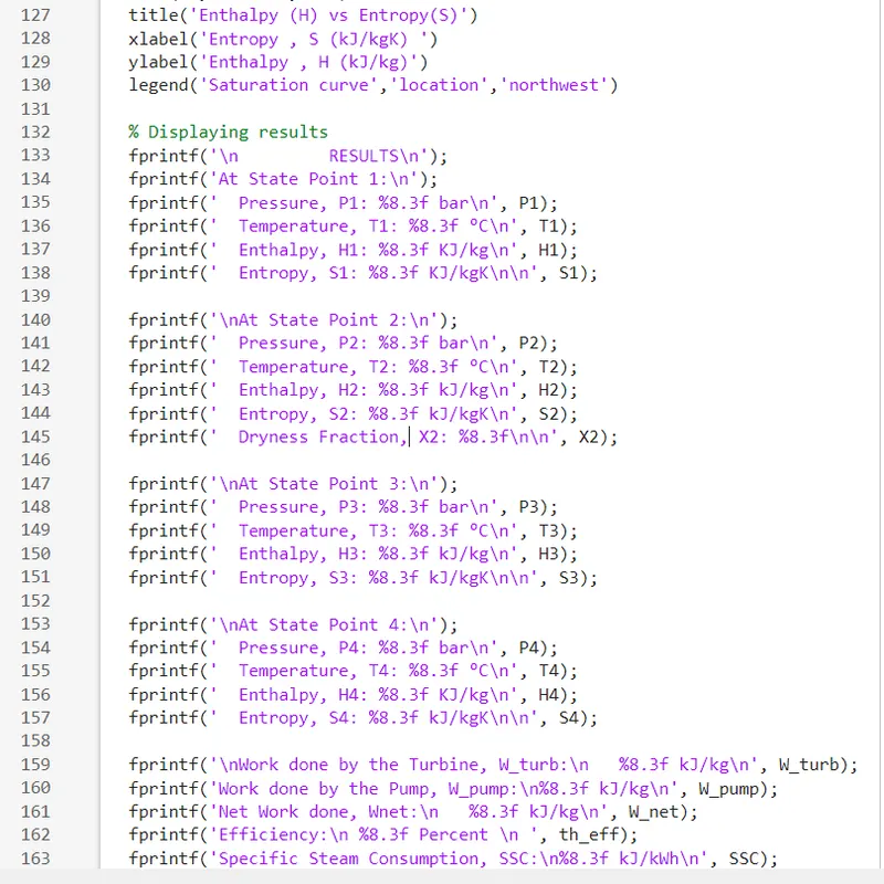
% Displaying results
fprintf('\n         RESULTS\n');
fprintf('At State Point 1:\n');
fprintf('  Pressure, P1: %8.3f bar\n', P1);
fprintf('  Temperature, T1: %8.3f °C\n', T1);
fprintf('  Enthalpy, H1: %8.3f KJ/kg\n', H1);
fprintf('  Entropy, S1: %8.3f KJ/kgK\n\n', S1);

fprintf('\nAt State Point 2:\n');
fprintf('  Pressure, P2: %8.3f bar\n', P2);
fprintf('  Temperature, T2: %8.3f °C\n', T2);
fprintf('  Enthalpy, H2: %8.3f kJ/kg\n', H2);
fprintf('  Entropy, S2: %8.3f kJ/kgK\n', S2);
fprintf('  Dryness Fraction, X2: %8.3f\n\n', X2);

fprintf('\nAt State Point 3:\n');
fprintf('  Pressure, P3: %8.3f bar\n', P3);
fprintf('  Temperature, T3: %8.3f °C\n', T3);
fprintf('  Enthalpy, H3: %8.3f kJ/kg\n', H3);
fprintf('  Entropy, S3: %8.3f kJ/kgK\n\n', S3);

fprintf('\nAt State Point 4:\n');
fprintf('  Pressure, P4: %8.3f bar\n', P4);
fprintf('  Temperature, T4: %8.3f °C\n', T4);
fprintf('  Enthalpy, H4: %8.3f KJ/kg\n', H4);
fprintf('  Entropy, S4: %8.3f kJ/kgK\n\n', S4);

fprintf('\nWork done by the Turbine, W_turb:\n   %8.3f kJ/kg\n', W_turb);
fprintf('Work done by the Pump, W_pump:\n%8.3f kJ/kg\n', W_pump);
fprintf('Net Work done, Wnet:\n   %8.3f kJ/kg\n', W_net);
fprintf('Efficiency:\n %8.3f Percent \n ', th_eff);
fprintf('Specific Steam Consumption, SSC:\n%8.3f kJ/kWh\n', SSC);
REPORT
Objectives :
- To create a Rankine Cycle simulator in MATLAB.
- To calculate the state point using function XSteam.
- To plot the T-S and H-S curves for given inputs in Rankine Cycle.
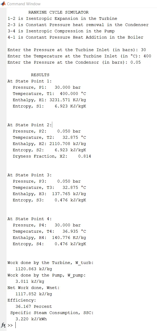
- To get output in the command window for each state point in the cycle.
Theory :
The Rankine cycle is an idealized thermodynamic cycle or heat engine. It is one of the vapor powered cycles derived from the Carnot cycle. A fuel is used to produce heat within a boiler , converting water into steam which then expands through a turbine producing useful work.
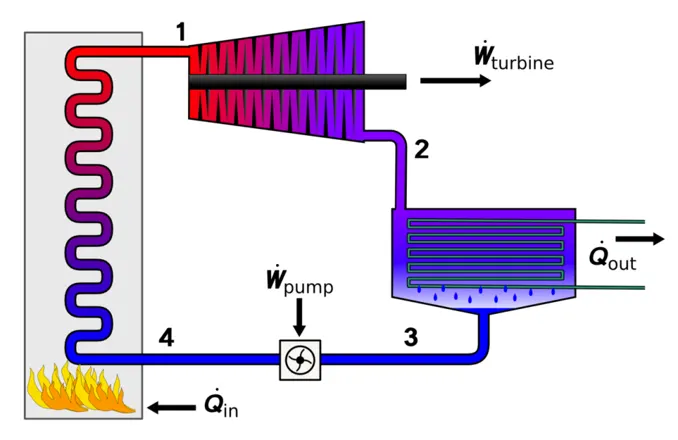
Process 1-2 : Isentropic expansion in a Turbine.
The dry saturated vapour expands through a turbine, generating power. This decreases the temperature and pressure of the vapour.
Process 2-3 : Constant pressure heat rejection in Condenser.
The vapor-liquid mixture leaving the turbine is condensed at low pressure. The pressure of the vapor is below atmospheric pressure, approaching the saturation pressure of the operating fluid.
Process 3-4 : Isentropic Compression in Pump.
The pressure of the condensate is raised in the feed pump and provided to the boiler.
Process 4-1 : Constant pressure heat addition in Boiler.
High pressure liquid enters the boiler and is heated to it’s saturation temperature. Further addition of energy causes evaporation of the liquid until it is fully converted to saturated steam or superheated steam.
All the four components of Rankine cycle are steady flow devices hence the process regarding this device can be evaluated as steady state process. The steady state flow energy equation per unit mass of steam reduces to:
(Qin - Qout) = (Win - Wout) = (he - hi)
The boiler and condenser are not involved in any mechanical work whereas pump and turbine are assumed to isentropic in nature while working throughout the cycle, then conservation of energy relation for each device can be expressed as:
Wpump = Win = h2 - h1 ,where h1 is enthalpy at P1 and h2 is enthalpy at P2
The heat added in boiler can be given as:
Qin = h3 - h2
The work which can be taken out of cycle from turbine is given as:
Wturb = Wout = h3 - h4
The heat removed from the condenser is given as:
Qout = h4 - h1
The thermal efficiency of Rankine cycle is given as:
ηth = Wnet/Win = Qnet/Qin = 1 - (Wout/Win) = 1 - (Qout/Qin)
Explanations :
- Xsteam data is used to extract steam and water properties of enthalpy , entropy at specific pressure and temperatures for saturated liquid, saturated vapour conditions.
- XSteam(‘h_TP’, t,p) is to find the enthalpy (H) at the conditons where teperature T is ‘t’ and Pressure P is ‘p’.
- XSteam(‘sL_T’, t) means to find the entropy (S) of a liquid (water) at a given temperature (T). Where the value passed it ’t’.
- The creation of Rankine cycle simulator starts with some input value which are required to calculate the other state point in cycle.
- Terms used in the code :
H1, H2, H3, H4 - enthalpy of the fluid at each state point.
S1, S2, S3, S4 - entropy of the fluid at each state point.
Sf and Sg - entropy of the fluid at saturated liquid and gaseous states. - All the details of the values used for plotting both the H-S and T-S graphs are printed as output in the command window.
Code:
Errors :
No complicated errors occurred while running the MATLAB program.
Outputs/ Plotted graphs :
Plots -
Results printed in the command window -
Conclusion :
- Created the Rankine cycle simulator for the given input, in which we have taken the data from XSteam function file.
- Plotted the required graphs and printed the needed output.
References :