Project 2 - Rankine cycle Simulator

Rankine cycle Simulator

Introduction:

The Rankine cycle is a thermodynamic cycle used in power plants and thermal systems to convert heat into mechanical work. It is commonly utilized in steam power plants and represents the idealized operation of a steam power cycle. The cycle consists of four main processes: expansion, heat addition, compression, and heat rejection.

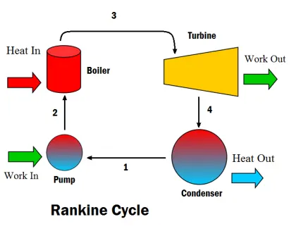
Explanation of the Rankine cycle:

1. Isentropic Expansion (1-2): The cycle starts with high-pressure, high-temperature steam entering a turbine. This steam expands isentropically (with no heat exchange) in the turbine, producing mechanical work and decreasing its pressure and temperature.

2. Constant Pressure Heat Addition (2-3): The expanded steam from the turbine enters a condenser where it is condensed at a constant pressure by rejecting heat to a cooling medium (typically water or air). This process reduces the steam's temperature and pressure, turning it into a saturated liquid.

3. Isentropic Compression (3-4): The saturated liquid from the condenser is further compressed using a pump. The pump increases the pressure of the liquid, requiring mechanical work input but with minimal temperature change.

4. Constant Pressure Heat Rejection (4-1): The compressed liquid from the pump enters a boiler or heat exchanger where it is heated at a constant pressure. Heat is supplied to the liquid, typically by burning fuel or using another heat source, causing it to evaporate and become high-temperature steam again.

The Rankine cycle is characterized by the following parameters and performance metrics:

• Pressure and temperature at various state points (1, 2, 3, 4) in the cycle.
• Enthalpy and entropy changes during each process.
• Work done by the turbine (Wt) and the pump (Wp).
• Net work output (W) obtained from the cycle.
• Heat added (qin) and heat rejected (qout) during the cycle.
• Thermal efficiency, calculated as the ratio of net work output to the heat added (eff = W/qin).
• Specific steam consumption (ssc), representing the mass flow rate of steam per unit of net work done.

By analyzing and optimizing the Rankine cycle, engineers can design efficient power plants and thermal systems that convert heat energy into useful work output.

%Rankine Cycle simulation

clear all
close all
clc

fprintf('Rankine Cycle\n');
fprintf('1-2 Isentropic Expansion in Turbine\n');
fprintf('2-3 Constant Pressure Heat Removal\n');
fprintf('3-4 Isentropic Compression in Pump\n');
fprintf('4-1 Constant Pressure Heat Addition in Boiler\n\n');

% Entering the input data for calculation of state points
%p1 = 60;       % Pressure at Turbine Inlet (bar)
%T1 = 800;      % Temperature at Turbine Inlet (°C)
%p2 = 7;        % Pressure at Condenser (bar)
disp('INPUTS');
p1 = input('Enter the Pressure at the Turbine Inlet (in bar): ');
T1 = input('Enter the Temperature at the Turbine inlet (in Degree C): ');
p2 = input('Enter the Pressure at the Condenser (in bar): ');


% Calculation of state point 1
h1 = XSteam('h_pT', p1, T1);   % Enthalpy at pressure and temperature 1
s1 = XSteam('s_pT', p1, T1);   % Entropy at pressure and temperature 1

% Calculation of state point 2
s2 = s1;                            % Isentropic expansion
sf2 = XSteam('sL_p', p2);           % Saturated liquid entropy at pressure 2
sg2 = XSteam('sV_p', p2);           % Saturated vapor entropy at pressure 2
x2 = (s2 - sf2) / (sg2 - sf2);      % Vapor fraction at state point 2
hf2 = XSteam('hL_p', p2);           % Saturated liquid enthalpy at pressure 2
hg2 = XSteam('hV_p', p2);           % Saturated vapor enthalpy at pressure 2
h2 = hf2 + x2 * (hg2 - hf2);        % Enthalpy at state point 2

% Calculation of state point 3
p3 = p2;                            % Constant pressure heat removal
s3 = XSteam('sL_p', p3);            % Saturated liquid entropy at pressure 3
h3 = XSteam('hL_p', p3);            % Saturated liquid enthalpy at pressure 3

% Calculation of state point 4
s4 = s3;                            % Isentropic compression
p4 = p1;                            % Constant pressure heat rejection
v3 = XSteam('vL_p', p3);             % Saturated liquid specific volume at pressure 3
Wp = v3 * (p4 - p3) * 100;           % Work done for pump
h4 = h3 - Wp;                        % Enthalpy at state point 4

% Work done in turbine for the Rankine cycle
Wt = h1 - h2;

% Net work done for the Rankine cycle
W = Wt - Wp;

% Heat addition to the system
qin = h1 - h4;

% Heat rejection from the system
qout = h2 - h3;

% Thermal efficiency of the Rankine cycle
eff = W * 100 / qin;

% Specific steam consumption (mass flow rate / net work done)
ssc = 3600 / W;

% Calculation of temperature at state points 2, 3, and 4
T3 = XSteam('Tsat_p', p3);       % Saturation temperature at pressure 3
T2 = T3;                        % Constant pressure heat addition
Cp4 = XSteam('Cp_ps', p4, s4);   % Specific isobaric heat capacity
Cv4 = XSteam('Cv_ps', p4, s4);   % Specific isochoric heat capacity
k = Cp4 / Cv4;
T4 = T3 / ((p3 / p4)^((k - 1) / k));  % Temperature at state point 4

% Calculation of other constants for saturated liquid and vapor
T6 = XSteam('Tsat_p', p1);          % Saturated temperature at pressure 1
s5 = XSteam('sL_p', p1);            % Saturated liquid entropy at pressure 1
s6 = XSteam('sV_p', p1);            % Saturated vapor entropy at pressure 1
h5 = XSteam('hL_p', p1);            % Saturated liquid enthalpy at pressure 1
h6 = XSteam('hV_p', p1);            % Saturated vapor enthalpy at pressure 1
T5 = T6;

% Plotting for saturation line
T = linspace(1, 560, 1000);
for i = 1:length(T)
    sf(i) = XSteam('sL_T', T(i));   % Saturated liquid entropy
    sg(i) = XSteam('sV_T', T(i));   % Saturated vapor entropy
    hf(i) = XSteam('hL_T', T(i));   % Saturated liquid enthalpy
    hg(i) = XSteam('hV_T', T(i));   % Saturated vapor enthalpy
end

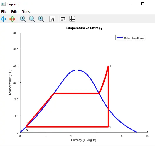
% Plotting T-S diagram for Rankine Cycle
figure(1)
hold on
plot(sf, T, 'color', 'b', 'linewidth', 2)
plot(sg, T, 'color', 'b', 'linewidth', 2)
plot([s1 s2], [T1 T2], 'color', 'r', 'linewidth', 3)
plot([s2 s3], [T2 T3], 'color', 'r', 'linewidth', 3)
plot([s3 s4], [T3 T4], 'color', 'r', 'linewidth', 3)
plot([s4 s5], [T4 T5], 'color', 'r', 'linewidth', 3)
plot([s5 s6], [T5 T6], 'color', 'r', 'linewidth', 3)
s_1 = linspace(s6, s1, 1000);
for j = 1:length(s_1)
    Tc(j) = XSteam('T_ps', p1, s_1(j));
end
plot(s_1, Tc, 'color', 'r', 'linewidth', 3)
text(s1 + 0.1, T1, '1')
text(s2 + 0.1, T2, '2')
text(s3, T3 - 20, '3')
text(s4, T4 + 20, '4')
title('Temperature vs Entropy')
xlabel('Entropy (kJ/kg-K)')
ylabel('Temperature (°C)')
legend('Saturation Curve')

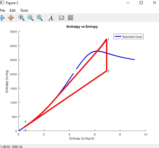
% Plotting H-S diagram for Rankine Cycle
figure(2)
hold on
plot(sf, hf, 'color', 'b', 'linewidth', 2)
plot(sg, hg, 'color', 'b', 'linewidth', 2)
plot([s1 s2], [h1 h2], 'color', 'r', 'linewidth', 3)
plot([s2 s3], [h2 h3], 'color', 'r', 'linewidth', 3)
plot([s3 s4], [h3 h4], 'color', 'r', 'linewidth', 3)
hc = linspace(h4, h5, 100);
for k = 1:length(hc)
    s_c(k) = XSteam('s_ph', p1, hc(k));
end
plot(s_c, hc, 'color', 'r', 'linewidth', 3)
plot([s5 s6], [h5 h6], 'color', 'r', 'linewidth', 3)
for l = 1:length(s_1)
    h_c(l) = XSteam('h_ps', p1, s_1(l));
end
plot(s_1, h_c, 'color', 'r', 'linewidth', 3)
text(s1 + 0.1, h1, '1')
text(s2 + 0.1, h2, '2')
text(s3, h3 - 100, '3')
text(s4, h4 + 200, '4')
title('Enthalpy vs Entropy')
xlabel('Entropy (kJ/kg-K)')
ylabel('Enthalpy (kJ/kg)')
legend('Saturation Curve')

% Displaying results in the command window
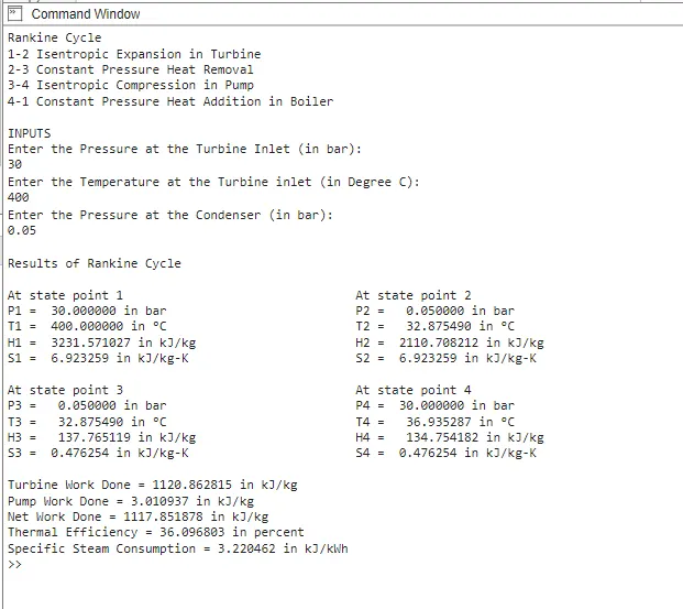
fprintf('\nResults of Rankine Cycle\n\n');
fprintf('At state point 1\t\t\t\t');
fprintf('At state point 2\n');
fprintf('P1 = %10f in bar\t\t\t\t', p1);
fprintf('P2 = %10f in bar\n', p2);
fprintf('T1 = %11f in °C\t\t\t\t', T1);
fprintf('T2 = %11f in °C\n', T2);
fprintf('H1 = %12f in kJ/kg\t\t\t', h1);
fprintf('H2 = %12f in kJ/kg\n', h2);
fprintf('S1 = %9f in kJ/kg-K\t\t\t', s1);
fprintf('S2 = %9f in kJ/kg-K\n', s2);
fprintf('\n');
fprintf('At state point 3\t\t\t\t');
fprintf('At state point 4\n');
fprintf('P3 = %10f in bar\t\t\t\t', p3);
fprintf('P4 = %10f in bar\n', p4);
fprintf('T3 = %11f in °C\t\t\t\t', T3);
fprintf('T4 = %11f in °C\n', T4);
fprintf('H3 = %12f in kJ/kg\t\t\t', h3);
fprintf('H4 = %12f in kJ/kg\n', h4);
fprintf('S3 = %9f in kJ/kg-K\t\t\t', s3);
fprintf('S4 = %9f in kJ/kg-K\n', s4);
fprintf('\n');
fprintf('Turbine Work Done = %f in kJ/kg\n', Wt);
fprintf('Pump Work Done = %f in kJ/kg\n', Wp);
fprintf('Net Work Done = %f in kJ/kg\n', W);
fprintf('Thermal Efficiency = %f in percent\n', eff);
fprintf('Specific Steam Consumption = %f in kJ/kWh\n', ssc);

Explanation:

1. The code begins by defining the known values for pressure (p1, p2, p3, p4) and specific volume at state point 3 (v3).
2. The next section of the code calculates the properties at state point 4, which occurs after isentropic compression from state 3. The pressure is constant at p4, and the work done by the pump (Wp) is calculated using the specific volume (v3). The enthalpy at state point 4 (h4) is determined by subtracting the work done by the pump from the enthalpy at state point 3.
3. The code then calculates the work done in the turbine for the Rankine cycle by subtracting the enthalpy at state point 2 (h2) from the enthalpy at state point 1 (h1).
4. Next, the net work done for the Rankine cycle is calculated by subtracting the work done by the pump (Wp) from the work done in the turbine (Wt).
5. The heat added to the system is calculated by subtracting the enthalpy at state point 4 (h4) from the enthalpy at state point 1 (h1).
6. Similarly, the heat rejected from the system is calculated by subtracting the enthalpy at state point 3 (h3) from the enthalpy at state point 2 (h2).
7. The thermal efficiency of the Rankine cycle is then calculated by dividing the net work done (W) by the heat added to the system (qin) and multiplying by 100.
8. The specific steam consumption, which represents the mass flow rate of steam per unit of net work done, is calculated by dividing 3600 (assumed mass flow rate in kg/hr) by the net work done (W).
9. The code proceeds to calculate the temperatures at state points 2, 3, and 4. The saturation temperature at pressure p3 (T3) is determined using the XSteam function. The temperature at state point 2 (T2) is assumed to be equal to T3 since heat is added at constant pressure. The specific heat capacities (Cp4 and Cv4) are calculated using the XSteam function. Finally, the temperature at state point 4 (T4) is calculated based on the isentropic compression process.
10. The code also calculates additional constants for the saturated liquid and vapor, such as the saturated temperature at pressure p1 (T6), the saturated liquid entropy at pressure p1 (s5), the saturated vapor entropy at pressure p1 (s6), the saturated liquid enthalpy at pressure p1 (h5), and the saturated vapor enthalpy at pressure p1 (h6). The temperature at state point 5 (T5) is assumed to be equal to T6.
11. Lastly, the code plots the T-S and H-S diagrams for the Rankine cycle and displays the results in the command window.

Outputs:

Errors faced:

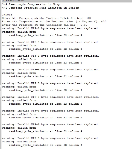
Here are few unexpected warnings poped up. Up enquiery it was found that in octave it was showing warnigs. Tried with online matlab problem was solves.

References:

1. Xsteam.m file

2. https://en.wikipedia.org/wiki/Rankine_cycle#:~:text=The%20Rankine%20cycle%20is%20an,heat%20source%20and%20heat%20sink.

3. https://www.youtube.com/watch?v=MQ13EepiG9Q