Project 2 - Rankine cycle Simulator

AIM: Create Rankine cycle simulator using the standard engg. Book.

OBJECTIVES:

1. Calculate the state points of the Rankine Cycle (any type of your choice) based on user inputs.
2. Then, plot the corresponding T-S and H-S plots for the given set of inputs.

INTRODUCTION: Rankine cycle is a power producing cycle which is widely used in steam-based power plants. The Rankine cycle produces high pressure and temperature steam which strikes the blade of the turbine and ultimately turbine rotates with high speed, further this turbine is coupled with a generator which converts the mechanical energy to electrical energy.

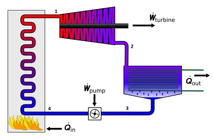
Heat energy is supplied to the system via a boiler where the working fluid (typically water) is converted to a high-pressure gaseous state (steam) in order to turn a turbine. After passing over the turbine the fluid is allowed to condense back into a liquid state as waste heat energy is rejected before being returned to boiler, completing the cycle. Friction losses throughout the system are often neglected for the purpose of simplifying calculations as such losses are usually much less significant than thermodynamic losses, especially in larger systems.

Process 1-2: Isentropic Expansion by Turbine

Turbine (1-2): Superheated steam enters into the Turbine and expands isentropically resulting in the production of work. The shaft of the turbine is connected to the generator. This results in the production of electricity i.e. Mechanical energy gets converted into electric energy. Work produced by the turbine,

W_T = m (h1−h2) K

Process 2-3: Constant Pressure Heat Rejection by Condenser

Condenser (2-3): The expanded vapour is then passed through a condenser, where it gets condensed and converts into liquid again. This liquid is again pumped to the boiler.

Q_R = m (h2−h3) K

Process 3-4: Isentropic Compression by the Pump

Pump (3-4): The water enters into the pump in a saturated state. Then the liquid is compressed isentropically until it meets the boiler pressure. Work done by the pump is,

W_P = m (h3−h4) K

Process 4-1: Constant Pressure Heat Addition by Boiler

Boiler (4-1): The water enters into the boiler as compressed and leaves as superheated from the boiler. Thus, the phase changes from liquid to vapour. The heat supplied by the boiler is

Q_A = m (h1−h4) K

The equations used for to get the work done are as below

Turbine Work (W_T):

W_T = H₁ - H₂

Pump Work (W_P):

W_P = H₄ - H₃

Net Work (W_NET):

W_NET = W_{T -} W_P

Thermal Efficiency (η):

η = W_NET/ (H_{1 -} H₄)

Back Work Ratio (BWR):

BWR = W_P /W_T

Specific Steam Conductivity (S.S.C):

S.S.C = 3600/W_T

Where,

H₁, H₂, H₃, H₄ are the enthalpy at the state points 1,2,3, and 4 respectively.

Explain of code:

Program initially displays the processes involved in Rankine cycle.

State 1 & 2 pressure and state 1 temperature are taken as input from user.

The values from the Xsteam library are extracted and the state values such as pressure, temperature, enthalpy and entropy are calculated.

Further the values of Turbine work, Pump work, Net_work ,Thermal Efficiency, Back Work Ratio and Specific Steam Conductivity are calculated.

All the calculated values are displayed in the command window.

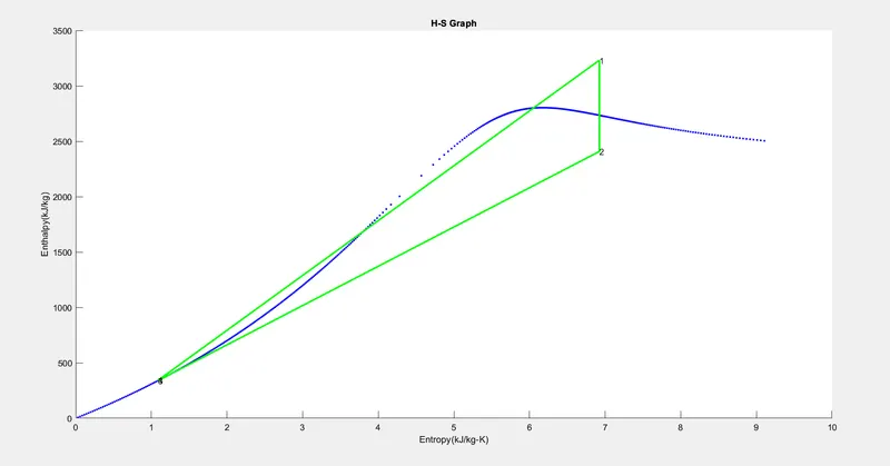
Finally, the T-S and H-S graph of the Rankine Cycle is plotted.

MAIN CODE:

clear all
close all
clc

disp('           RANKINE CYCLE SIMULATOR           ')
disp(' 1-2 is Isentrpic expansion in Turbine');
disp(' 2-3 is Heat Rejection by condenser at constant Pressure');
disp(' 3-4 is Isentropic compression in Pump');
disp(' 4-1 id Heat addition by Boiler at constant Pressure');
disp(' ')

% Required Inputs by user
P1 = input("Enter the Pressure at the Turbine inlet(in bar) = ");
T1 = input("Enter the Temperature at the Turbine inlet(in degree celcius) = ");
P2 = input("Enter the Pressure at the condenser(in bar) = ");
disp(' ')

% Calculating the state values

% At state point 1
H1 = XSteam('h_pT',P1,T1);   % Enthalpy Point
S1 = XSteam('s_pT',P1,T1);   % Entropy Point
H_liquid1 = XSteam('hL_p',P1);  % Liquid enthalpy at point 1
H_gas1 = XSteam('hV_p',P1);     % Gas enthalpy at point 2
S_liquid1 = XSteam('sL_p',P1);  % Liquid entropy at point 1
S_gas1 = XSteam('sV_p',P1);     % Gas entropy at point 2
T_saturation1 = XSteam('Tsat_p',P1);  % Saturation Temperature at point 1

% At state point 2
S2 = S1;    % Entropy at point 1-2 is constant coz the isentropic compression
S_liquid2 = XSteam('sL_p',P2);   % Entropy at liquid point 2
S_gas2 = XSteam('sV_p',P2);      % Entropy at gas point 2
d_f = (S2 - S_liquid2)/(S_gas2 - S_liquid2);    % Dryness-fraction at state point 2
H_liquid2 = XSteam('hL_p',P2);   % Enthalpy at liquid point 2
H_gas2 = XSteam('hV_p',P2);      % Enthalpy at gas point 2
H2 = H_liquid2 + d_f * (H_gas2 - H_liquid2);    % Enthalpy at state point 2
T2 = XSteam('T_ph',P2,H2);       % Temperature at point 2
T_saturation2 = XSteam('Tsat_p',P2);   % Saturation Temperature at point 2

% At state point 3
P3 = P2;    % Constant pressure at P3 and P2
T3 = T2;    % Constant Temperature at T3 and T2 
H3 = H_liquid2;  % Enthalpy H3 is same as Liquid enthalpy 2
S3 = S_liquid2;  % Entropy S3 is same as Liquid entropy 2

% At state point 4
P4 = P1;     % Constant pressure at P4 and P1 
S4 = S3;     % Constant Entropy at S4 and S4 coz isentropic expansion 
T4 = XSteam('T_ps',P4,S4);   % Temperature at point 4 from book
H4 = XSteam('H_ps',P4,S4);   % Enthalpy at point 4 from book

%Calculating Work, Back Work Ratio, Specific Steam Conductivity and Efficiency

% Work done by Turbine
W_turbine = H1 - H2;

% Work done by Pump
W_pump = H4 - H3;

% Net work done
W_net = W_turbine - W_pump;

% Thermal Efficiency of the Rankine cycle 
Effinciency = (W_net/(H1 - H4))*100;

% Back work ratio
B_W_R = W_pump/W_turbine;

% Specific Steam conductivity
SSC = 3600/W_turbine;

% Displying results
% state point 1
disp('            RESULT          ')
disp('state point 1')
fprintf('P1 is = %f Bar \n',P1);
fprintf('T1 is = %f deg celcius \n',T1);
fprintf('H1 is = %f Kj/Kg \n',H1);
fprintf('S1 is = %f Kj/Kg K \n \n',S1);

% Values of state point 2
disp('state point 2')
fprintf('P2 is = %f Bar \n',P2);
fprintf('T2 is = %f deg celcius \n',T2);
fprintf('H2 is = %f Kj/Kg \n',H2);
fprintf('S2 is = %f Kj/Kg k \n \n',S2);

% Values of state point 3
disp('state point 3')
fprintf('P3 is = %f Bar \n',P3);
fprintf('T3 is = %f deg celcius \n',T3);
fprintf('H3 is = %f Kj/Kg \n',H3);
fprintf('S3 is = %f Kj/Kg k \n \n',S3);

% Values of state point 4
disp('state point 4')
fprintf('P4 is = %f Bar \n',P4);
fprintf('T4 is = %f deg celcius \n',T4);
fprintf('H4 is = %f Kj/Kg \n',H4);
fprintf('S4 is = %f Kj/Kg k \n \n',S4);

% Turbine work
fprintf('Turbine work = %f Kj/Kg \n',W_turbine);

% Pump Work
fprintf('Pump Work = %f Kj/Kg \n',W_pump);

% Net Work
fprintf('Net Workdone = %f Kj/Kg \n',W_net);

% Thermal Efficiency
fprintf('Thermal Efficiency = %f \n',Effinciency);

% Specific Steam Conductivity
fprintf('Specific Steam Conductivity = %f Kg/KW h \n',SSC);

% Back Work ratio
fprintf('Back work ratio = %f \n',B_W_R);


%plotting of T-S curve
t = linspace(0,373.5,200);
figure(1)
hold on

for i = 1:length(t)
plot(XSteam('sL_T',t(i)),t(i),'g.')
plot(XSteam('sV_T',t(i)),t(i),'g.')
end

plot([S1 S2],[T1 T2],'linewidth',2,'color','b')
text(S1,T1,'1','FontSize',10)
if d_f>1
T3 = T_saturation2;
plot([S2 S_gas2 S3 S4],[T2 T_saturation2 T3 T4],'linewidth',2,'color','r')
T2 = T_saturation2;
text(S2,T2,'2','FontSize',10)
text(S3,T3,'3','FontSize',10)
else
plot([S2 S3 S4],[T2 T3 T4],'linewidth',2,'color','b')
text(S2,T2,'2','FontSize',10)
text(S3,T3,'3','FontSize',10)
end

n = linspace(T1,T2,500);
for i = 1:length(n)
plot(XSteam('s_pT',P1,n(i)),n(i),'.','linewidth',2,'color','r')
end

plot([S_liquid1 S_gas1],[T_saturation1 T_saturation1],'linewidth',2,'color','b')
text(S_liquid1,T_saturation1,'4','FontSize',10)
xlabel('Entropy(kJ/kg-K)')
ylabel('Temperature(k)')
title('T-S Graph')


%Plotting of H-S Curve
figure(2) 
hold on
for i = 1:length(t)
 plot(XSteam('sL_T',t(i)),XSteam('hL_T',t(i)),'b.')
 plot(XSteam('sV_T',t(i)),XSteam('hV_T',t(i)),'b.')
end
plot([S1 S2 S3 S4 S1],[H1 H2 H3 H4 H1],'linewidth',2,'color','g')
text(S1,H1,'1','FontSize',10)
text(S2,H2,'2','FontSize',10)
text(S3,H3,'3','FontSize',10)
text(S4,H4,'4','FontSize',10)
xlabel('Entropy(kJ/kg-K)')
ylabel('Enthalpy(kJ/kg)')
title('H-S Graph')

Results from code:

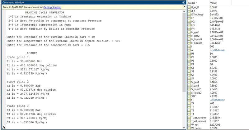
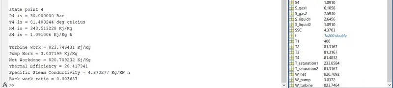
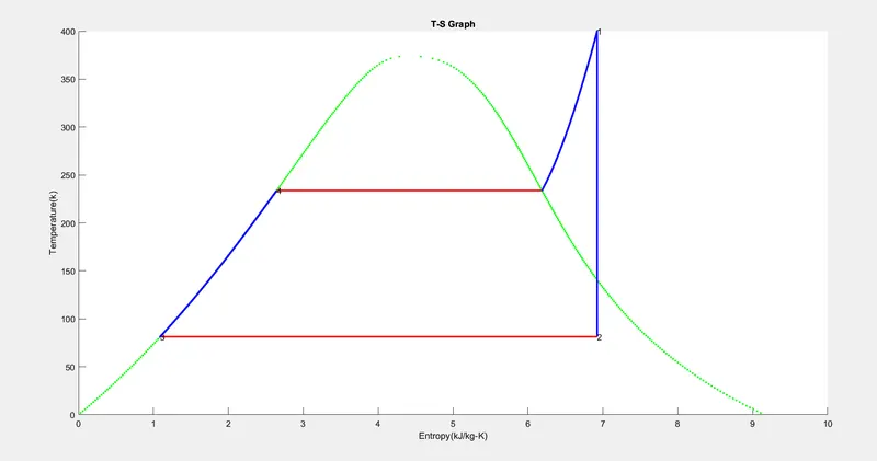
T-S Graph:

H-S Graph:

CONCLUSION:

The values of Pressure, Temperature, Enthalpy and Entropy for different state points and also the Work, Efficiency, Back work ratio and Specific steam conductivity was calculated and Also the graph of T-S and H-S for Rankine Cycle was plotted.

References:

https://en.wikipedia.org/wiki/Rankine_cycle

What is Rankine Cycle - Steam Turbine Cycle - Definition (thermal-engineering.org)