PROJECT REQUIREMENTS:


1. Create a Rankine Cycle Simulator using MATLAB.
2. Calculate the state points of the Rankine Cycle based on user inputs.
3. Plot the corresponding T-s and h-s Diagram.
4. The working of a rankine cycle simulator.

%*. What is rakine cycle?

The rakine cycle is the thermodynamic cycle by which heat engines like, steam engines, steam turbine, allows mechanical work to be extracted from the fluid as it moves between a heat source and heat sink. This cycle is mostly used by powerplants such as coal powered power plants and nuclear reactors.

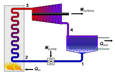
In this process, the water is being pumped from lake or any huge water storage tank to the boiler. with the help of fuel, the water is boiled at high temperature within boiler to convert into the steam, later the steam exapand into the turbine blades which produce work. Then, exapnded steam goes to condeser to get condense and become water again. The water then again sent to pump and cycle repeats.

Thus, the cycle is divided in 4 processes.

1. Process 1-2: The working fluid is pumped from low pressure to high pressure, for which energy is used in terms of pump. Process 1-2 is known as isentropic compression.

2. Process 2-3: The high pressure fluid enters into the boiler and heated at high temperarue at constant pressure which converts the water into dry saturated vapor. Gas or coal is used as fuel for heating up the fluid or water. Process 2-3 is known as Constant pressure heat addition.

3.Process 3-4: The dry saturated vapor,then, expands into the turbine and produce power. So, the pressure and temperature reduce and it condenses the vapor. Process 3-4 is known as isentropic exapnsion.

4. Process 4-1: The wet vapor goes into the condeser which finally condense at constant pressure and become saturated liquid. Process 4-1 is known as constant pressure heat rejection.


%*> Formula's to calculate output parameters.

Turbine Work Wt: H1-H2
Pump Work Wp: H4-H3
Q(in)= H1-H4
Q(out)=H2-H3

W(net): Wt-Wp

THERMAL EFFICIENCY = Wt/Q(in)

Specific Stem Consuption(S.S.C):

S.S.C = 3600/W(net)

Back work Ratio:

B.W.R=Q(in))/Q(out)


clear all
close all
clc

% Rankine cycle project simulator
% 'fprintf' is used to printout required output as shown.

fprintf('RANKINE CYCLE PROJECT SIMULATOR \n ')
fprintf('1-2 is Isentropic expansion in the turbine \n')
fprintf(' 2-3 is Constant pressure heat rejection by the condenser\n')
fprintf(' 3-4 is Isentropic compression in the pump\n')
fprintf(' 4-1 is Constant pressure heat addition by the boiler\n')


% data for the state point 1
p1=30;
t1=400;
h1=XSteam('h_pT',p1,t1);
s1=XSteam('s_pT',p1,t1);

% 'fprintf' is used to printout required output as shown.

fprintf('\n\n Results for state 1')
fprintf('\n p1 is : %f bar',p1)
fprintf('\n T1 is:%f deg celcius',t1)
fprintf('\n h1 is :%f KJ/KG',h1)
fprintf('\n s1 is:%f KJ/KgK',s1)


%taking data for state 2 from Xsteam file.
p2=0.05;
s2=s1;

% 'fprintf' is used to printout required output as shown.

t2=XSteam('T_ps',0.05,s2);
sf2=XSteam('sL_p',p2);
sg2=XSteam('sV_p',p2);
hf2=XSteam('hL_p',p2);
hg2=XSteam('hV_p',p2);

x2=((s2-sf2)/(sg2-sf2));
h2=hf2+(x2*(hg2-hf2));
v2=XSteam('v_ph',p2,h2);

% 'fprintf' is used to printout required output as shown.

fprintf('\n\n Results for state 2')
fprintf('\n p2 is : %f bar',p2)
fprintf('\n T2 is:%f deg celcius',t2)
fprintf('\n h2 is :%f KJ/KG',h2)
fprintf('\n s2 is:%f KJ/KgK',s2)


% taking data for state point 3 from XSteam file

t3=t2;
p3=p2;
s3=XSteam('sL_P',p3);
h3=XSteam('hL_T',s3);
v3=XSteam('v_ph',p3,h3);

% 'fprintf' is used to printout required output as shown.

fprintf('\n\n Results for state 3')
fprintf('\n p3 is : %f bar',p3)
fprintf('\n T3 is:%f deg celcius',t3)
fprintf('\n h3 is :%f KJ/KG',h3)
fprintf('\n s3 is:%f KJ/KgK',s3)

%taking data for state point 4 from Xsteam file
s4=s3;
p4=p1;
v4=v3;
h4=XSteam('h_ps',p4,s4);
t4=XSteam('T_ps',h4,s4);

% 'fprintf' is used to printout required output as shown.

fprintf('\n\n Results for state 4')
fprintf('\n p4 is : %f bar',p4)
fprintf('\n T4 is:%f deg celcius',t4)
fprintf('\n h4 is :%f KJ/KG',h4)
fprintf('\n s4 is:%f KJ/KgK',s4)

%taking data for state point 5 from Xsteam file
p5=p4;
t5=XSteam('Tsat_p',p5);
h5=XSteam('hL_T',t5);
s5=XSteam('sL_p',p5);

% 'fprintf' is used to printout required output as shown.

fprintf('\n\n Results for state 5')
fprintf('\n p5 is : %f bar',p5)
fprintf('\n T5 is:%f deg celcius',t5)
fprintf('\n h5 is :%f KJ/KG',h5)
fprintf('\n s5 is:%f KJ/KgK',s5)

%taking data for state point 6 from Xsteam file
t6=t5;
p6=XSteam('psat_T',t5);
s6=XSteam('sV_T',t6);
h6=XSteam('hV_T',t6);

% 'fprintf' is used to printout required output as shown.

fprintf('\n\n Results for state 6')
fprintf('\n p6 is : %f bar',p6)
fprintf('\n T6 is:%f deg celcius',t6)
fprintf('\n h6 is :%f KJ/KG',h6)
fprintf('\n s6 is:%f KJ/KgK',s6)

%net work
% finding work output's using rankine cycle formula

w_turbine=h1-h2;
w_pump=h4-h3;
w_net=w_turbine-w_pump;
q_in=h1-h4;
q_out=h2-h3;

%specific stem consption
s.s.c=3600/w_net;

% back work ratio
BWR=q_in/q_out;

%thermal efficiency
Eff=(w_net/q_in)*100;

fprintf('\n w_turbine is : %f kj/kg',w_turbine)
fprintf('\n w_punp is: %f kj/kg',w_pump)
fprintf('\n w_net is : %f kj/kg',w_net)
fprintf('\n s.s.c is:%f kh/kWh',s.s.c)
fprintf('\n thermal eff:%f percent',Eff)


t=linspace(0,400,1000);
for i=1:length(t)
    s_1(i)=XSteam('sL_T',t(i));
end

for j=1:length(t)
    s_2(j)=XSteam('sV_T',t(j));
end

for i= 1:length(t)
    h_1(i)=XSteam('hL_T',t(i));
end

for j=1:length(t)
    h_2(j)=XSteam('hV_T',t(j));

end

%plotting T-S diagram

figure(1)
hold on
plot([s_1 s_2],[t t])
plot([s1 s2 s3 s4 s5 s6 s1], [t1 t2 t3 t4 t5 t6 t1])

%using 'text' command to locate process point on graph

text(s1,t1,'1')
text(s2,t2,'2')
text(s3,t3,'3')
text(s4,t4,'4')
text(s5,t5,'5')
text(s6,t6,'6')

%titling and labeling the graph
title('RANKINE CYCLE T-S DIAGRAM')
xlabel('Entropy(kj/kgk)')
ylabel('temperature(k)')
axis([0 9 0 500])

%plotting H_S diagram
%using 'text' command to locate process point on graph

figure(2)
hold on
plot([s_1 s_2],[h_1 h_2])
plot([s1 s2 s3 s4 s5 s6 s1], [h1 h2 h3 h4 h5 h6 h1])
text(s1,h1,'1')
text(s2,h2,'2')
text(s3,h3,'3')
text(s4,h4,'4')
text(s5,h5,'5')
text(s6,h6,'6')

%titling and labeling the graph
title('RANKINE CYCLE H-S DIAGRAM')
xlabel('Entrophy(kj/kgK)')
ylabel('Enthalphy(kj/kg)')
axis([0 9 0 3200])

% RANKINE CYCLE SIMULATOR COMPLETE