Project 2 - Rankine cycle Simulator

Aim: To understand the Rankine Cycle and simulate it using MATLAB.

Objective:

1. To Simulate a Rankine cycle using Matlab.
2. Extracting Steam and water properties from the Xstram file.
3. To calculate the state variables at each point
4. Calculating every cycle's state point based on user inputs.
5. To plot the T-S and H-S graphs.

Introduction:

The Rankine cycle closely describes the process by which steam engines commonly found in thermal power generation plants harness the thermal energy of a fuel or other heat source to generate electricity. Possible heat sources include the combustion of fossil fuels such as coal, natural gas, and oil, the use of mined resources for nuclear fission, renewable fuels like biomass and ethanol, or energy capture of natural sources such as concentrated solar power and geothermal energy. Common heat sinks include ambient air above or around a facility and bodies of water such as rivers, ponds, and oceans.

The ability of a Rankine engine to harness energy depends on the relative temperature difference between the heat source and heat sink. The greater the differential, the more mechanical power can be efficiently extracted out of heat energy, as per Carnot's theorem.

Processes and Working :

There are four processes in the Rankine cycle :

1. Process 1-2: Isentropic Expansion in the turbine
2. Process 2-3: Constant pressure Heat rejection in the condenser
3. Process 3-4: Isentropic compression in the pump
4. Process 4-1: Constant pressure heat addition in the boiler

• Rankine cycle efficiency ηR is

Code program and explantion:

disp(' RANKINE CYCLE ');  
                                 
disp('1-2 is Constant pressure heat addition in the boiler');

disp('2-3 is Isentropic Expansion in the Turbine');

disp('3-4 is Constant pressure heat removal in the Condenser');

disp('4-1 is Isentropic compression in the pump');

p1 = input('nValue of pressure at turbine inlet, p1(in bar) = ');
T1 = input('nValue of temperature at turbine inlet, T1(in degree.C) = ');
p2 = input('nValue of pressure at condenser inlet, p2(in bar) = ');
 

% At State 1

h1 = XSteam('h_pT', p1, T1);        
s1 = XSteam('s_pT', p1, T1);      

% At State 2

s2 = s1;                                         
sf2= XSteam('sL_p', p2);            
sg2 = XSteam('sV_p', p2);          
x2 = (s2-sf2)/(sg2-sf2);
hf2 = XSteam('hL_p', p2);           
hg2 = XSteam('hV_p', p2);
h2 = hf2 + (x2*(hg2-hf2));

% At State 3

p3 = p2;                            
s3= XSteam('sL_p', p3);
h3 = XSteam('hL_p', p3);

% At State 4
s4 = s3;
p4 = p1;

% Work done by turbine
Wt = h1 - h2;

% Work done to run pump
v3 = XSteam('vL_p', p3);
Wp = v3*(p4 - p3)*100;
h4 = h3 + Wp;

%Net work

Wnet = Wt - Wp;

%Heat into the system

Qin = h1 - h4;

%Heat out of the system

Qout = h2 - h3;

%Thermal efficiency

thermal_eff = (Wnet/Qin)*100;

%Specific Steam Consumption

%SSC = mass flow rate/power

SSC = (3600/Wnet);

% Back Work ratio

BW = (Wp/Wt)


% Calculation of Temperatures at the state points

T3 = XSteam('Tsat_p', p3);
T2 = T3;
Cp4 = XSteam('Cp_ps', p4, s4);
Cv4 = XSteam('Cv_ps', p4, s4);
k = Cp4/Cv4;
T4 = T3/((p3/p4)^((k-1)/k));

%Calculating Temperature, Entropy and Enthalpy at the vapour and liquid line for plotting

T6 = XSteam('Tsat_p', p1);
s5 = XSteam('sL_p', p1);
s6 = XSteam('sV_p', p1);
h5 = XSteam('hL_p', p1);
h6 = XSteam('hV_p', p1);
T5 = T6;


%Plotting the saturation curve

T = linspace(1,375,1000);
for i = 1:length(T)

sf(i) = XSteam('sL_T', T(i));
sg(i) = XSteam('sV_T', T(i));
hf(i) = XSteam('hL_T', T(i));
hg(i) = XSteam('hV_T', T(i));
end

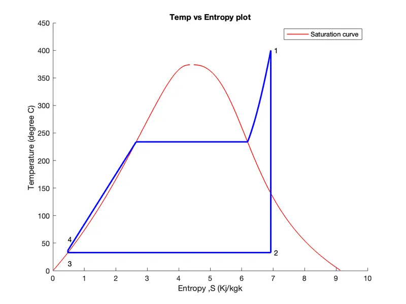
%Plotting T-s diagram

figure(1)

hold on

plot(sf, T, 'r','linewidth',1)
plot(sg, T, 'r','linewidth',1)
plot([s1 s2], [T1 T2], 'b', 'linewidth', 2)
plot([s2 s3], [T2 T3] ,'b', 'linewidth', 2)
plot([s3 s4], [T3 T4], 'b', 'linewidth', 2)
plot([s4 s5], [T4 T5], 'b', 'linewidth', 2)
plot([s5 s6], [T5 T6], 'b', 'linewidth', 2)

sc1 = linspace(s6, s1, 1000);
for l = 1:length(sc1)
 Tc1(l) = XSteam('T_ps', p1, sc1(l));
end

plot(sc1, Tc1, 'b', 'linewidth', 2)
text(s1+0.1, T1, '1')
text(s2+0.1, T2, '2')
text(s3, T3-20, '3')
text(s4, T4+20, '4')
title('Temp vs Entropy plot')
xlabel('Entropy ,S (Kj/kgk')
ylabel('Temperature (degree C) ')
legend('Saturation curve')


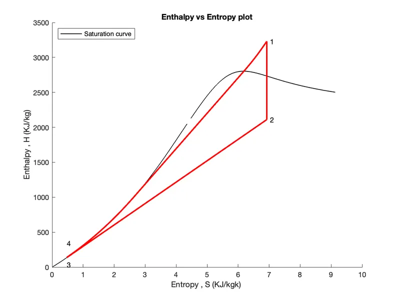
%Plotting h-s diagram

figure(2)

hold on

plot(sf, hf, 'k', 'linewidth', 1)
plot(sg, hg, 'k',  'linewidth', 1)
plot([s1 s2], [h1 h2], 'r', 'linewidth', 2)
plot([s2 s3], [h2 h3], 'r', 'linewidth', 2)
plot([s3 s4], [h3 h4], 'r', 'linewidth', 2)

hc = linspace(h4, h5, 100);

for r = 1:length(hc)
sch(r) = XSteam('s_ph', p1, hc(r));
end

plot(sch,hc, 'r', 'linewidth', 2)
plot([s5 s6], [h5 h6], 'r', 'linewidth', 2)

for m = 1:length(sc1)
hc1(m) = XSteam('h_ps', p1, sc1(m));
end

plot(sc1, hc1, 'r', 'linewidth', 2)
text(s1+0.1, h1, '1')
text(s2+0.1, h2, '2')
text(s3, h3-100, '3')
text(s4, h4 +200, '4')
title('Enthalpy vs Entropy plot')
xlabel('Entropy , S (KJ/kgk) ')
ylabel('Enthalpy , H (KJ/kg)')
legend('Saturation curve','location','northwest')



% Displaying the Results in the Command Window:

disp('Results');

p1 = p1;
T1 = T1;
p2 = p2;
disp('At stage point 1');
n1 = sprintf('P1 is %.3f bar',p1);
disp(n1);
n2 = sprintf('T1 is %.3f C',T1);
disp(n2);
n3 = sprintf('h1 is %.3f kJ/kg',h1);
disp(n3);
n4 = sprintf('s1 is %.3f kJ/kgK',s1);
disp(n4);
disp('At stage point 2');
n11 = sprintf('P2 is %.3f bar',p2);
disp(n11);
n21 = sprintf('T2 is %.3f C',T2);
disp(n21);
n31 = sprintf('h2 is %.3f kJ/kg',h2);
disp(n31);
n41 = sprintf('s2 is %.3f kJ/kgK',s2);
disp(n41);
disp('At stage point 3');
n12 = sprintf('P3 is %.3f bar',p3);
disp(n12);
n22 = sprintf('T3 is %.3f C',T3);
disp(n22);
n32 = sprintf('h3 is %.3f kJ/kg',h3);
disp(n32);
n42 = sprintf('s3 is %.3f kJ/kgK',s3);
disp(n42);
disp('At stage point 4');
n13 = sprintf('P4 is %.3f bar',p4);
disp(n13);
n23 = sprintf('T4 is %.3f C',T4);
disp(n23);
n33 = sprintf('h4 is %.3f kJ/kg',h4);
disp(n33);
n43 = sprintf('s4 is %.3f kJ/kgK',s4);
disp(n43);
n14 = sprintf('Wt is %.3f kJ/kg',Wt);
disp(n14);
n15 = sprintf('Wp is %.3f kJ/kg',Wp);
disp(n15);
n16 = sprintf('Wnet is %.3f kJ/kg',Wnet);
disp(n16);
n17 = sprintf('Thermal_efficiency is %.2f Percent',thermal_eff);
disp(n17);
n18 = sprintf('SSC is %.2f kg/kWh',SSC);
disp(n18);
n19 = sprintf('Back work ratio is %.3f ',BW);
disp(n19);

1. The program for the input of pressure (in bars) at state point 1 (the turbine inlet), the temperature at the same point (degrees Celsius), and pressure at the condenser inlet (point 2).
2. XStream data is used to extract steam and water properties of enthalpy, entropy at a specific pressure, and temperatures for sat liquid, sat vapor conditions, etc.
3. The program calculates all the Rankine cycle state points using these inlets and data from Xsteam.
4. The XStream data operates as follows: h1 = XStream ('h pT', p1, T1); it returns the water's enthalpy in bar and degC at the specified pressure and temperature.
5. After analyzing the plots of Rankine cycles and extracting data from an Xsteam file, Sf and sg, hf and hg, where f and g stand for saturated liquid and saturated vapor, respectively, are calculated.
6. After learning about the Rankine cycle, we use thermodynamic relations to further find state points and extract their data from XStream as we extract data.
   
7. For plotting purposes, T, s, and h are extracted at the liquid and vapor lines after the fourth point to account for the variation you see in the plot.
8. For saturated liquid and saturated gas, the saturation curve is plotted in red in T-S, and in H-S, it is black.
9. Using the plot command and specifying all of the labels, linewidth, colors, and titles, a plot of T vs s and h vs s is generated from all the points obtained from the program.
10. As the user's input for the above-mentioned inputs changes, the plot also changes.

Output:

	

 RANKINE CYCLE 

1-2 is Constant pressure heat addition in the boiler
2-3 is Isentropic Expansion in the Turbine
3-4 is Constant pressure heat removal in the Condenser
4-1 is Isentropic compression in the pump

nValue of pressure at turbine inlet, p1(in bar) = 30
nValue of temperature at turbine inlet, T1(in degree.C) = 400
nValue of pressure at condenser inlet, p2(in bar) = 0.05

Results
At stage point 1
P1 is 30.000 bar
T1 is 400.000 C
h1 is 3231.571 kJ/kg
s1 is 6.923 kJ/kgK
At stage point 2
P2 is 0.050 bar
T2 is 32.875 C
h2 is 2110.708 kJ/kg
s2 is 6.923 kJ/kgK
At stage point 3
P3 is 0.050 bar
T3 is 32.875 C
h3 is 137.765 kJ/kg
s3 is 0.476 kJ/kgK
At stage point 4
P4 is 30.000 bar
T4 is 36.935 C
h4 is 140.776 kJ/kg
s4 is 0.476 kJ/kgK
Wt is 1120.863 kJ/kg
Wp is 3.011 kJ/kg
Wnet is 1117.852 kJ/kg
Thermal_efficiency is 36.17 Percent
SSC is 3.22 kg/kWh
Back work ratio is 0.003

Results:

Following calculations of the Heat Engine's performance, the following observations were made:

Net Work = 1120.863kJ/kg

Thermal Efficiency = 36.17%

Back Work Ratio = 0.003

The Rankine Cycle's T-S and H-S performance curves were plotted.

Conclusion:

The Rankine Cycle simulation has been done using Matlab.