Project 2 - Rankine cycle Simulator

Aim -

• To Develop a basic program that calculates the state points
• To add the thermodynamic relation to get the points inbetween the state variables.
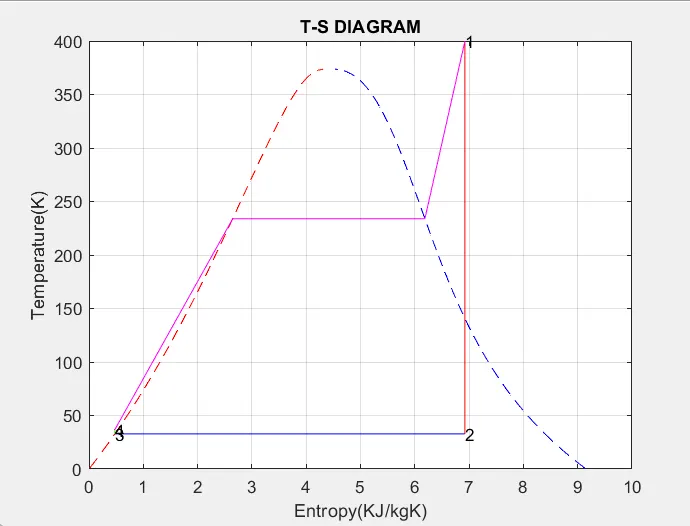
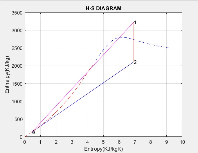
• To plot rankine cycle on T-s and H-s curve.

THEORY :

The Rankine cycle is the fundamental operating cycle of all power plants where an operating fluid is continuously evaporated and condensed. The selection of operating fluid depends mainly on the available temperature range.

The Rankine cycle operates in the following steps:

1-2 Isentropic Expansion. The vapor is expanded in the turbine, thus producing work which may be converted to electricity. In practice, the expansion is limited by the temperature of the cooling medium and by the erosion of the turbine blades by liquid entrainment in the vapor stream as the process moves further into the two-phase region. Exit vapor qualities should be greater than 90% to increase the life of turbine blade.

2-3 Isobaric Heat Rejection. The vapor-liquid mixture leaving the turbine is condensed at low pressure, usually in a surface condenser using cooling water. In well designed and maintained condensers, the pressure of the vapor is well below atmospheric pressure, approaching the saturation pressure of the operating fluid at the cooling water temperature.

3-4 Isentropic Compression. The pressure of the condensate is raised in the feed pump. Because of the low specific volume of liquids, the pump work is relatively small and often neglected in thermodynamic calculations.

4-1 Isobaric Heat Transfer. High pressure liquid enters the boiler from the feed pump and is heated to the saturation temperature . Further addition of energy causes evaporation of the liquid until it is fully converted to saturated steam.

Code Explanation -

• The Program begins with clear all, close all, clc to erase the workspace and plots..
• Input variables p1,t1,p2 are given by input command whose values are entered in command window while executing the Program.
• State-1, Values for Enthalpy & Entropy are extracted as a function of Pressure & Temperature.
• h_pT, s_pT, hL_p, sV_p etc.... are the default variables whose value is stored in XSteam file.
• Similarly, all the variables for all states are extracted using a suitable format.[**The Formulae for the State Variables and other depending factors are referred from Power Plant Reference Books.]
• Pressure, Temperature, Enthalpy, Entropy for all the State Variables are Extracted as a function of the dependent variable from the XSteam File.
• State 2 is a Condenser inlet where the High-Pressure Steam is converted into Low-Pressure Water and hence Dryness Fraction, Enthalpy & Entropy for Saturated Vapour & Saturated Water are considered to Calculate the Specific Enthalpy.
• State-3 The water is condensed back to its Saturation Temperature and fed to the Pump, This temperature of water at the exit of the Condenser and entry of Pump is the same.
• State-4 This is Constant Pressure Heat addition, hence pressure is equal to p1, but the temperature increases on heating at Constant Pressure & Constant Volume as our Entropy remains same and hence Cp/Cv=gamma is considered to find temperature T4.
• Finally Work done and Heat Evolved & SSC are calculated by basic formulae.
• To plot the Saturation Curve, a Temperature range is defined using linspace command and for the overall length of this Temperature values of Enthalpy and Entropy are calculated at every temperature point. The Break in the Saturation Curve separates the Liquid Phase & Vapour Phase.
• Now all the necessary data is found out, Plotting is done for both T-S & H-S curves using the plot commands. Annotations are assigned using text command.
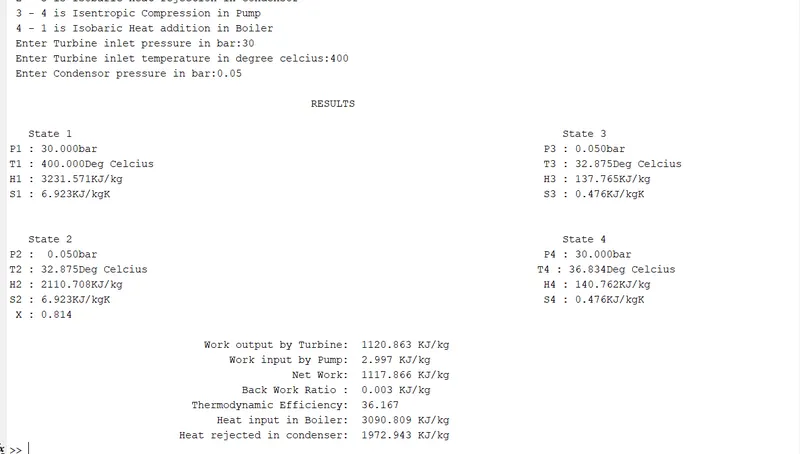
• Results of the Cycle Simulation is displayed over Comand window using fprintf command.

Results -

1.

2.

3.

Conclusion

• Rankine cycle is a power generating cycle.
• Superheating increase the thermal efficiency of cycle.
• It is the most practical cycle.

Code -

%Rankine Simulator 
clear all
close all
clc

disp('Rankine Cycle Simulator')
disp('1 - 2 is Isentropic Expansion in Turbine')
disp(' 2 - 3 is Isobaric Heat rejection in Condensor')
disp(' 3 - 4 is Isentropic Compression in Pump')
disp(' 4 - 1 is Isobaric Heat addition in Boiler')

%Inputs 
p1 = input(' Enter Turbine inlet pressure in bar:')
t1 = input(' Enter Turbine inlet temperature in degree celcius:')
p2 = input(' Enter Condensor pressure in bar:')

%State Point 1 
s1 = XSteam('s_pT',p1,t1);   %Entropy at state 1
h1 = XSteam('h_pT',p1,t1);   %Enthalpy at state 1

%State Point 2 
s2 = s1;                   %Entropy at state 2
t2 = XSteam('Tsat_p',p2);
sf2=XSteam('sL_p',p2);  %Entropy at liquid state
sg2=XSteam('sV_p',p2);  %Entropy at gaseous state
hf2=XSteam('hL_p',p2);  %Enthalpy at liquid state
hg2=XSteam('hV_p',p2);  %Enthalpy at gaseous state

x2=(s2-sf2)/(sg2-sf2);  %dryness fraction factor
h2=hf2+(x2*(hg2-hf2));  %Enthalpy at state 2

%State Point 3 
p3 = p2; 
t3 = t2; 
s3 = XSteam('sL_T',t3);  %Entropy at state 2
v3f= XSteam('vL_p',p3);
h3=hf2;                  %Enthalpy at state 3

%State Point 4 
p4 = p1;
s4 = s3;                    %Entropy at state 4
h4 = XSteam('h_ps',p4,s4);  %Enthalpy at state 4
cp4 = XSteam('CpL_p',p3);
cv4 = XSteam('CvL_p',p3);
gamma = (cp4/cv4);

% To calculate the t4
% p4^(1-gamma)*t4^gamma = p3^(1-gamma)*t3^gamma
t4 = (t3*((p3/p4)^((1-gamma)/gamma)));

% Calculation

%Work done by turbine
wt = h1 - h2;

%Work done by pump
wp = h4 - h3;

%Net Work done
w_net = wt - wp;

%Back  work ratio
BWR = wp/wt

%Heat injected in boiler
q_in = h1 - h4;

%Heat rejected in condensor
q_out = h2 - h3;

%Thermal Efficiency
n = w_net/q_in;
np = n*100;

%Plot for Temperature vs Entropy
figure(1)

%plot for liquid and vapour saturation curves
t = linspace(0,550,600);

for i = 1:length(t)
    s_l(i) = XSteam('sL_T',t(i));
end

for i = 1:length(t)
    s_v(i) = XSteam('sV_T',t(i));
end

plot(s_l,t,'--','color','r')
hold on
plot(s_v,t,'--','color','b')
grid on


%plot for Work done by turbine
plot([s1,s2],[t1,t2],'color','r')
hold on
title('T-S DIAGRAM')
xlabel('Entropy(KJ/kgK)')
ylabel('Temperature(K)')

%plot for heat rejected in condensor
plot([s2,s3],[t2,t3],'color','b')
hold on

%plot for work done by pump
plot([s3,s4],[t3,t4],'color','g')
hold on

%plot for heat injected by boiler
tp = XSteam('TSat_p',p4);
sp = XSteam('sL_T',tp);
plot([s4,sp],[t4,tp],'color','m')
hold on

tq = tp;     %For Straight line 
sq = XSteam('sV_T',tq);
plot([sp,sq],[tp,tq],'color','m')
hold on

plot([sq,s1],[tq,t1],'color','m')
hold on

%Indicate states with numbers
text(s1,t1,'1');
text(s2,t2,'2');
text(s3,t3,'3');
text(s4,t4,'4');

%Plot for enthalpy vs entropy
figure(2)

plot([s1,s2],[h1,h2],'color','r')
grid on
title('H-S DIAGRAM')
xlabel('Entropy(KJ/kgK)')
ylabel('Enthalpy(KJ/kg)')
hold on

plot([s2,s3],[h2,h3],'color','b')
hold on
plot([s3,s4],[h3,h4],'color','g')
hold on
plot([s4,s1],[h4,h1],'color','m')
hold on

%plot for liqiuid and vapour saturation curve

t = linspace(0,550,600);
for j = 1:length(t)
    h_l(j) = XSteam('hL_T',t(j));
end

for j = 1:length(t)
    h_v(j) = XSteam('hV_T',t(j));
end


plot(s_l,h_l,'--','color','r')
hold on
plot(s_v,h_v,'--','color','b')

%Indicate states with numbers
text(s1,h1,'1');
text(s2,h2,'2');
text(s3,h3,'3');
text(s4,h4,'4');

%Results output
fprintf('\n%55s','RESULTS')
fprintf('\n \n%10s %84s \n','State 1','State 3');
fprintf('%s %6.3f%s %74s %.3f%s \n','P1 :',p1,'bar','P3 :',p3,'bar');
fprintf('%s %.3f%s %65s %.3f%s \n','T1 :',t1,'Deg Celcius','T3 :',t3,'Deg Celcius');
fprintf('%s %8.3f%s %70s %.3f%s \n','H1 :',h1,'KJ/kg','H3 :',h3,'KJ/kg');
fprintf('%s %.3f%s %72s %.3f%s \n','S1 :',s1,'KJ/kgK','S3 :',s3,'KJ/kgK');

fprintf('\n \n%10s %84s \n','State 2','State 4');
fprintf('%s %6.3f%s %74s %.3f%s \n','P2 :',p2,'bar','P4 :',p4,'bar');
fprintf('%s %.3f%s %65s %.3f%s \n','T2 :',t2,'Deg Celcius','T4 :',t4,'Deg Celcius');
fprintf('%s %8.3f%s %70s %.3f%s \n','H2 :',h2,'KJ/kg','H4 :',h4,'KJ/kg');
fprintf('%s %.3f%s %72s %.3f%s \n ','S2 :',s2,'KJ/kgK','S4 :',s4,'KJ/kgK');
fprintf('%s %0.3f%s \n ','X :',x2);

fprintf('\n \n%55s %.3f %s \n','Work output by Turbine: ',wt,'KJ/kg');
fprintf('%55s %.3f %s \n','Work input by Pump: ',wp,'KJ/kg');
fprintf('%55s %.3f %s \n','Net Work: ',w_net,'KJ/kg');
fprintf('%55s %.3f %s \n','Back Work Ratio : ',BWR,'KJ/kg');
fprintf('%55s %.3f \n','Thermodynamic Efficiency: ',np);
fprintf('%55s %.3f %s \n','Heat input in Boiler: ',q_in,'KJ/kg');
fprintf('%55s %.3f %s \n','Heat rejected in condenser: ',q_out,'KJ/kg');