Challenge

Project 2 - Rankine cycle Simulator

MMadhurjya Gogoi1 Aug 2022

Aim:

From the given inputs,creation of Rankine cycle simulator and to extract the steam and water properties from XSteam data.

Objectives:

To create a Rankine cycle simulator.
To calculate the state point using XSteam function.
To plot T vs S and H vs S curve for the given inputs.
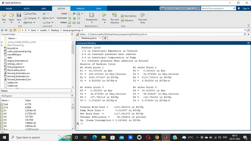
To get output in command window for each point in cycle.

Rankine cycle:

It is one of the vapor powered cycle.This cycle is somewhat different than gas powered cycle in which working fluid remained gas throughout the entire cycle,In vapor powered cycle the working fluid is water.Mainly rankine cycle is an idealized thermodynamic cycle or heat engine in which a fuel is used to produce heat within a boiler,converting water into steam which expand through a turbine producing useful work.

The process in rankine cycle are:

Isentropic expansion in turbine.
Constant pressure heat rejection in condenser.
Isentropic compression in a pump.
Constant pressure heat addition in boiler.

Working of the rankine cycle simulator:

In process 1-2,The superheated vapor enters the turbine, where it expands isentropically and generate power.This decreases the temperature and pressure of the vapor,and some condensation may occur.
Process 2-3,The steam enters the condenser,At this state steam is usually a saturated liquid vapor mixture with a high quality.Steam is condensed at constant pressure in the condenser,which is basically a large heat exchanger by rejecting heat to a cooling medium.
Process 3-4,Water enters the pump at this state as saturated liquid and is compressed isentropically to operate the pressure of the boiler.The pressure of the condensate is raised in the feed pump,because of the low specific volume of liquids,the pump work is relatively small and often neglected in thermodynamic calculation.
Process 4-1,High pressure liquid enters the boiler from the feed pump and is heated to the saturation temperature.Further,addition of energy causes evaporation of the liquid untill it is fully converted to saturated steam or super heated vapor.

Main code:

clear all
close all
clc
% Rankine Cycle Simulator

fprintf(' Rankine Cycle\n ')
fprintf('1-2 is Isentropic Expansion in Turbine\n')
fprintf(' 2-3 is constant pressure heat removal\n')
fprintf(' 3-4 is Isentropic Compression in Pump \n')
fprintf(' 4-1 Constant pressure Heat addition in Boiler\n')

% Entering the input data for calculation of state points
p1 = 44;        %Pressure at Turbine Inlet
T1 = 538;       %Temperature at Turbine Inlet
p2 = 5.83;      %Pressure at Condenser

% Taking data from Xsteam file for State point 1
h1 = XSteam('h_pT', p1, T1);        % Enthaply at pressure and Temp 1
s1 = XSteam('s_pT', p1, T1);        % Entropy at pressure and Temp 1

% Taking data from Xsteam file for State point 2
s2 = s1;                            % Because of Isentropic Expansion
sf2 = XSteam('sL_p', p2);           % Saturated liquid entropy at pressure 2
sg2 = XSteam('sV_p', p2);           % Saturated vapour entropy at pressure 2
x2 = (s2-sf2)/(sg2-sf2);            % Vapour Fraction at state point 2
hf2 = XSteam('hL_p', p2);           % Saturated liquid Enthalpy at pressure 2
hg2 = XSteam('hV_p', p2);           % Saturated vapour Enthalpy at pressure 2
h2 = hf2 + (x2*(hg2-hf2));          % Enthalpy at state point 2

% Taking data from Xsteam file for state point 3
p3 = p2;                            % Constant Pressure heat removal process
s3 = XSteam('sL_p', p3);            % Saturated liquid entropy at Pressure 3
h3 = XSteam('hL_p', p3);            % Saturated liquid Enthalpy at Pressure 3

% Taking data from Xsteam file for State point 4
s4 = s3;                            % Isentropic Compression process
p4 = p1;                            % Constant Pressure heat rejection

% Work done in Turbine for the rankine cycle
W_T = h1-h2;

% Work done required for pump
v3 = XSteam('vL_p',p3);             % Saturated Liquid Vapour at pressure 3
W_P = v3*(p4-p3)*100;               % Work done for pump
h4 = h3 - W_P;                      % Enthalpy at State point 4

% Net work done for Rankine Cycle
W_net = W_T - W_P;

% Heat Addition to System
Q_in = h1-h4;

% Heat Rejection from System
Q_out = h2-h3;

% Thermal Efficiency of Rankine Cycle
T_eff = (W_net/Q_in)*100;

%specific steam consumption  = (Mass flow rate / Net work done)
Sp_S = (3600/W_net);

% Calculation of Temperature at All state Point 2, 3 and 4
T3 = XSteam('Tsat_p',p3);           % Saturation Temperature at Pressure 3
T2 = T3;                            % Becuase of Constant Pressure Heat addition
Cp4 = XSteam('Cp_ps',p4,s4);        % Specific isobaric heat capacity
Cv4 = XSteam('Cv_ps',p4,s4);        % Specific isochoric heat capacity
z = Cp4/Cv4;
T4 = T3/((p3/p4)^((z-1)/z));        % Temperature at State point 4

% Calculation of Other constant for saturated liquid and Vapour
T6 = XSteam('Tsat_p', p1);          % Saturated Temperature at Pressure 1
s5 = XSteam('sL_p', p1);            % Saturated Liquid entropy at pressure 1
s6 = XSteam('sV_p', p1);            % Saturated Vapour entropy at Pressure 1
h5 = XSteam('hL_p', p1);            % Saturated Liquid Enthalpy at Pressure 1
h6 = XSteam('hV_p', p1);            % Saturated Vapour Enthalpy at pressure 1
T5 = T6;

%Plotting for Saturation Line
T = linspace(1,600,1000);
for i = 1:length(T)
    sf(i) = XSteam('sL_T' ,T(i));   % Saturated Liquid Entropy
    sg(i) = XSteam('sV_T' ,T(i));   % Saturated Vapour Entropy
    hf(i) = XSteam('hL_T' ,T(i));   % Saturated Liquid Enthalpy
    hg(i) = XSteam('hV_T' ,T(i));   % Saturated Vapour Enthalpy
    
end

% Plotting T-S Diagram for Rankine Cycle
figure(1)
hold on
plot(sf,T,'color','b','linewidth',2)
plot(sg,T,'color','b','linewidth',2)
plot([s1 s2],[T1 T2], 'color', 'r', 'linewidth',3)
plot([s2 s3],[T2 T3], 'color', 'r', 'linewidth',3)
plot([s3 s4],[T3 T4], 'color', 'r', 'linewidth',3)
plot([s4 s5],[T4 T5], 'color', 'r', 'linewidth',3)
plot([s5 s6],[T5 T6], 'color', 'r', 'linewidth',3)
s_1 = linspace(s6,s1,1000);
for k = 1:length(s_1)
    Ta(k) = XSteam('T_ps',p1,s_1(k));
end
plot(s_1,Ta,'color','r','linewidth',3)
text(s1+0.1, T1, '1')
text(s2+0.1, T2, '2')
text(s3, T3-20, '3')
text(s4, T4+20, '4')
title('Temperature Vs Entropy')
xlabel('Entropy (Kj/kg-k)')
ylabel('Temeperature (Deg. Celcius)')
legend('Saturation Curve')

% Plotting H-S Diagram for Rankine Cycle
figure(2)
hold on
plot(sf,hf,'color','b','linewidth',2)
plot(sg,hg,'color','b','linewidth',2)
plot([s1 s2],[h1 h2],'color','r','linewidth',3)
plot([s2 s3],[h2 h3],'color','r','linewidth',3)
plot([s3 s4],[h3 h4],'color','r','linewidth',3)
hc = linspace(h4,h5,100);
for z = 1:length(hc)
    s_a(z) = XSteam('s_ph',p1,hc(z));
end
plot(s_a,hc,'color','r','linewidth',3)
plot([s5 s6],[h5 h6],'color','r','linewidth',3)
for l = 1:length(s_1)
    h_c(l) = XSteam('h_ps',p1,s_1(l));
end
plot(s_1,h_c,'color','r','linewidth',3)
text(s1+0.1,h1,'1')
text(s2+0.1,h2,'2')
text(s3,h3-100,'3')
text(s4,h4+200,'4')
title('Enthalpy Vs Entropy')
xlabel('Entropy (Kj/kg-k)')
ylabel('Enthalpy (KJ/Kg)')
legend('Saturation Curve')

% Displaying Results in Command window
disp('Results of Rankine Cycle')
fprintf('At state point 1\t\t\t\t\t')
fprintf('At state Point 2\n')
fprintf('P1 = %10f in Bar\t\t\t\t',p1);
fprintf('P2 = %10f in Bar\n',p2);
fprintf('T1 = %11f in Deg.Celcius\t\t',T1);
fprintf('T2 = %11f in Deg.Celcius\n',T2);
fprintf('H1 = %12f in KJ/Kg\t\t\t',h1);
fprintf('H2 = %12f in KJ/Kg\n',h2);
fprintf('S1 = %9f in KJ/Kg-k\t\t\t',s1);
fprintf('S2 = %9f in KJ/Kg-k\n',s2);
fprintf('\n')
fprintf('At state point 3\t\t\t\t\t')
fprintf('At state Point 4\n')
fprintf('P3 = %10f in Bar\t\t\t\t',p3);
fprintf('P4 = %10f in Bar\n',p4);
fprintf('T3 = %11f in Deg.Celcius\t\t',T3);
fprintf('T4 = %11f in Deg.Celcius\n',T4);
fprintf('H3 = %12f in KJ/Kg\t\t\t',h3);
fprintf('H4 = %12f in KJ/Kg\n',h4);
fprintf('S3 = %9f in KJ/Kg-k\t\t\t',s3);
fprintf('S4 = %9f in KJ/Kg-k\n',s4);
fprintf('\n')
fprintf('Turbine Work Done = %14f in KJ/Kg\n',W_T)
fprintf('Pump Work Done = %15f in KJ/Kg\n',W_P)
fprintf('Net Work Done  = %17f in KJ/Kg\n',W_net)
fprintf('Thermal Efficiency = %13f in percent\n',T_eff)
fprintf('Sp. Steam Consumption = %f in KJ/Kw\n',Sp_S)

Code explaination:

The program starts with clc,clear all,close all.
The program requires the input of pressure (in bar) at state point 1(turbine inlet),temperature at same state point 1(deg celcius),pressure at state point 2(condenser).
Then we are using xsteam function file for reading state points.
With the help of those inlets and xSteam data,the programe calculates all the state points and the rankine cycle.
As the process from 1-2 is isentropic compression the entropy at point 1 is equal to point 2.The term (s_pT,p1,T1) refers to entropy at pressure and temperature at point 1,and (h_pT,p1,T1) refers to enthalpy at point 1.
The term 'sg' and 'sf' are reffered to saturated vapor and saturated liquid entropy respectively.
Simlilarly 'hg' and 'hf' are reffered to saturated vapor and saturated liquid enthalpy respectively.
As we extract the data,we use thermodynamic relation further to find the state points and extract their data from xSteam.
The net workdone for rankine cycle,workdone in turbine,workdone to run the pump,heat in and heat out are calculated using standard thermodynamic relation.
Thermal Efficiency and SSC of the rankine cycle is calculated.
Then the temperature at each point of cycle is calculated using input taken from start of the program and data taken from xSteam file.For given temperature range, lower to higher entropy points are calculated to create the T-S plot .Similarly,another for loop is used to create the saturation curve in each point.
Plot of T vs S and H vs S are created from all the points obtained from the programe .
Saturation curve is plotted in red for saturated liquid and saturated vapor.
Results are displayed in command window.

Ouput:

For the Input given in the challenge:

Figure1: Inlet pressure in turbine = 30 bar

Inlet temperature in turbine = 400 deg.cel

Pressure in condenser = .05 bar

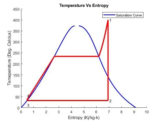
Figure2:

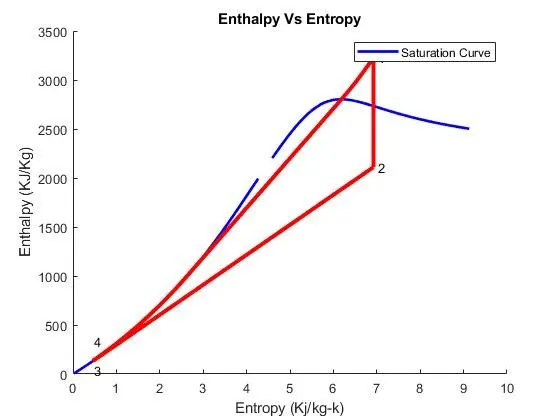
Figure3. Result in the Command windows(screenshot)

References:-

Project 2 - Rankine cycle Simulator

Ship work like this
in your own course.

Talk to a career counsellor

Ship work like thisin your own course.

Talk to a career counsellor

Ship work like this
in your own course.