Project 2 - Rankine cycle Simulator

Aim:

To write a code for Ranckine cycle with the help of given XSteam table code and plot T-S and H-S diagram for the gie input data.

Code:

clear all
close all
clc

%rancline cycle
disp('Process 1-2 : Isentropic Expansion in the turbine');
disp('Process 2-3 : Constant Pressure Heat Rejection by the Condensor');
disp('Process 3-4 : Isentropic expansion in the pump');
disp('process 4-1 : Constant pressure Heat addision in the Boiler');

%Given Data
%Initial Temperacture in celsius : Turbne inlet
t1 = 400; 
%Initial Pressure in bar : Turbne inlet
p1 = 30;
%Condensor Inlet Presure in bar/ Turbne outlet
p2 = 0.05;

%stage 1 Calculaction
h1 = XSteam('h_pt',p1,t1);
s1 = XSteam('s_pt',p1,t1);

%stage 2
%Entropy 
s2 = s1;
gama = 1.4;
t2 = t1*((p2/p1)^(1-(1/gama)));
h2 = XSteam('h_pt',p2,t2);

%stage 3
p3 = p2;
s3 = XSteam('sl_p',p3);
h3 = XSteam('hl_p',p3);

%stage 4
s4 = s3;
p4 = p1;

%net work done = turbine work output power-pump input power 
%turebine work
turbine_work = h1-h2;
v3 = XSteam('vl_p',p3);

%pump input\output power
pump_Work = v3*(p4-p3)*100;
h4 = h3+pump_Work;

%over all work
Net_work = turbine_work-pump_Work;
Qin = h1-h4;
Qout = h2-h3;

%we know t1 at stage 1. to find t at other stages
%we know p3=0.05
t3 = XSteam('tsat_p',p3);

%specific heat at t4
Cp = XSteam('cp_ps',p4,s4);
%specific volume at t4
Cv = XSteam('cv_ps',p4,s4);
k = Cp/Cv;
t4 = t3/((p3/p4)^((k-1)/k));

%to plot H-S and T-S diagram we need t5,t6,h5,h6,s5,s6
t6 = XSteam('tsat_p',p1);
s5 = XSteam('sl_p',p1);
s6 = XSteam('sv_p',p1);
h5 = XSteam('hl_p',p1);
h6 = XSteam('hv_p',p1);
t5 = t6;

%over-all thermal efficiency of the cycle
Thermal_efficiency = (Net_work/Qin)*100;

%to ind Back Work Ractio

bwr = (h4-h3)/(h2-h1);

%to calculate entropy and entholpy for saturaction curve

temp = linspace(1,375,1000);
for i = 1:length(temp)
    sf(i) = XSteam('sl_t',temp(i));
    sg(i)= XSteam('sv_t',temp(i));
    hf(i) = XSteam('hl_t',temp(i));
    hg(i) = XSteam('hv_t',temp(i));
end


%T-S Plotting
figure(1)
hold on
plot(sf,temp,'color','r','LineWidth',1,'color','b');
plot(sg,temp,'color','r','LineWidth',1,'color','y');
plot([s1 s2],[t1 t2],'color','r','LineWidth',2,'Marker','*')
plot([s2 s3],[t2 t3],'color','r','LineWidth',2,'Marker','*')
plot([s3 s4],[t3 t4],'color','r','LineWidth',2,'Marker','*') 
plot([s4 s5],[t4 t5],'color','r','LineWidth',2,'Marker','*')
plot([s5 s6],[t5 t6],'color','r','LineWidth',2,'Marker','*')
plot([s6 s1],[t6 t1],'color','r','LineWidth',2,'Marker','*')
xlabel('Entopy')
ylabel('Temperacture in C')
title('Temperacture vs Entropy plot')
legend('Saturaction curve at liquide state','saturaction curve at vapour state','T-S curve')

%H-S Plotting
figure(2)
hold on
plot([sg sf],[hg hf],'LineWidth',1,'Color','b');
plot([s1 s2],[h1 h2],'color','r','LineWidth',2,'Marker','*')
plot([s2 s3],[h2 h3],'color','r','LineWidth',2,'Marker','*')
plot([s3 s4],[h3 h4],'color','r','LineWidth',2,'Marker','*')
plot([s4 s5],[h4 h5],'color','r','LineWidth',2,'Marker','*')
plot([s5 s6],[h5 h6],'color','r','LineWidth',2,'Marker','*')
plot([s6 s1],[h6 h1],'color','r','LineWidth',2,'Marker','*')
xlabel('Entholpy')
ylabel('Entopy')
title('Entholpy vs Entropy plot')
legend('Saturaction curve','H-S curve')

Explanaction:

• clear all, close all, clc commend helps to clear all all the data stored in work space,close all files related to matlab and clear all data in commend prompt.

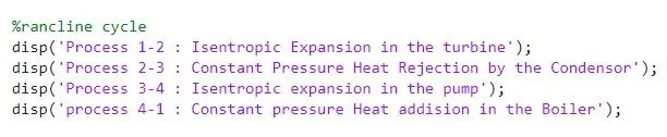
• these syntex gives the detail about hole ranckine cycle
• the Respective inputs given to the variables:T1 = 400°C , P1 = 30 bar, P2 = 0.05bar and air constant gamma = 1.4.
• then the entropy and enthalpy value for process 1-2 ; values are taken respect to P1,T1 from XSteam table.
• t2 is calculated with the formula and the respective entholpy value taken from XSteam file.
• since p3 = p2 , the entropy and entholpy ate taken from Xsteam file respect to p3.
• frome P-V and T-S diagram s4 = s3 and p4 = p1 the values are taken.

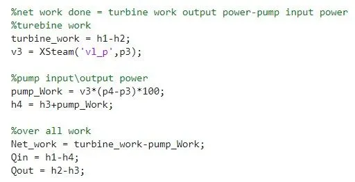
• to calculate the net work output we need to reduce the power input for the pump to the turbine output.
• using the formula the values are calculated
• Qin is the difference between heat h1 to h4 and Qout is the difference between h2 to h3.
• t3 is calculated by the XSteam table with respect to p3.

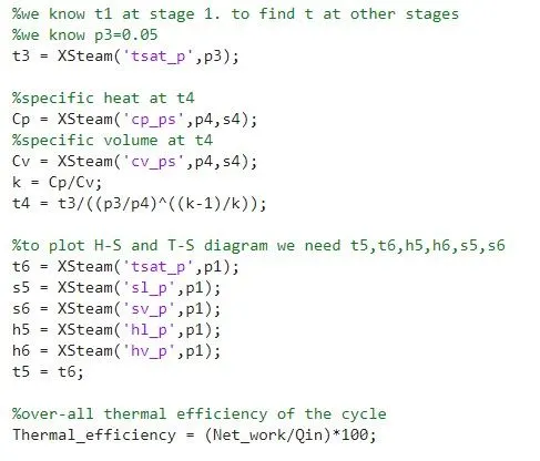
• to plot the P-V and H-S diagram the respective values for all the points are calculated by XSteam table as shown in figure
• the thermal efficiency is calculated by the formula ratio of net work done by the cycle to the heat input to the system to the times 100.
• to plot the saturaction curve we need to find the entropy and entholpy value for saturaction point for the number of time with the respective state which is vapour and liquied.

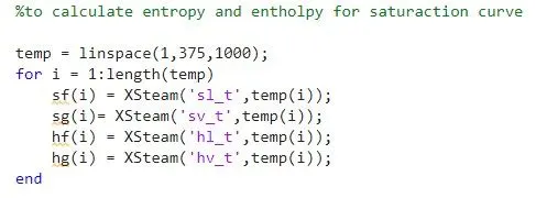
• As shown in the figure a for loop is created to find the entropy and entholypy in vapour and liquied state with the times of temp(i).
• the plots diagram is done by the value calculated at each stage.
• P-V and H-S diagram has attached to the file.

Commends:

• i strugle while ploting the saturaction curve because i did not give the sf(i)- i times in each vale insted of that i gave sf = XSteam('sl_t',temp(i)); by doing these for each loop all the values are re-assigned to the same variable. By doing these i did not get the plot. After refering the old probles i got to know the mistake that i have done.
• while doing the H-S plot diagram initialy i got confused with the satureaction curve after consulting with the instructor and re-reading the question asked in the chalange the answer is already has shown as model and i did it correctly.