Project 2 - Rankine cycle Simulator

THEORY:

RANKINE CYCLE: THE IDEAL CYCLE FOR VAPOR POWER CYCLES

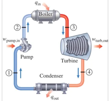
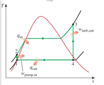
The Rankine cycle, which is the ideal cycle for vapor power plants. The ideal Rankine cycle does not involve any internal irreversibilities and consists of the following four processes:

1-2 Isentropic compression in a pump

2-3 Constant-pressure heat addition in a boiler

3-4 Isentropic expansion in a turbine

4-1 Constant-pressure heat rejection in a condenser

Water enters the pump at state l as saturated liquid and is compressed isentropically to the operating pressure of the boiler. The water temperature increases somewhat during this isentropic compression process due to a slight decrease in the specific volume of water. The vertical distance between states 1 and 2 on the T-s diagram is greatly exaggerated for clarity.

Water enters the boiler as a compressed liquid at state 2 and leaves as a superheated vapor at state 3. The boiler is basically a large heat exchanger where the heat originating from combustion gases, nuclear reactors, or other sources is transferred to the water essentially at constant pressure. The boiler, together with the section where the steam is superheated (the super-heater), is often called the steam generator.

The superheated vapor at state 3 enters the turbine, where it expands isentropically and produces work by rotating the shaft connected to an electric generator. The pressure and the temperature of steam drop during this process to the values at state 4, where steam enters the condenser. At this state, steam is usually a saturated liquid-vapor mixture with a high quality. Steam is condensed at constant pressure in the condenser, which is basically a large heat exchanger, by rejecting heat to a cooling medium such as a lake, a river, or the atmosphere. Steam leaves the condenser as saturated liquid and enters the pump, completing the cycle. In areas where water is precious, the power plants are cooled by air instead of water. This method of cooling, which is also used in car engines, is called dry cooling.

Remembering that the area under the process curve on a T-s diagram represents the heat transfer for internally reversible processes, we see that the area under process curve 2-3 represents the heat transferred to the water in the boiler and the area under the process curve 4-1 represents the heat rejected in the condenser. The difference between these two (the area enclosed by the cycle curve) is the net-work produced during the cycle.

Equations

(qin-qout)+(win-wout)=he-hi (kJ/kg)

Pump(q=0)

wpump.in=h2-h1

wpump.in=v(P2-P1)

h1=h@P1v=va=vf@P1

Boiler(w=0):

Turbine(q=0):

Condensor(w=0):

qin=h3-h2

wturb.out=h3-h4

qout=h4-h1

`eta`nth=Wnet/qin =1-(qout/qin)

Wnet=qin-qout=Wturb,out-Wpump,in

RANKINE CYCLE:IDEAL CYCLE FOR VAPOUR POWER CYCLE

Process 1-2: Reversible adiabatic expansion process in the steam turbine

Process 2-3: Constant pressure heat transfer process in the condenser

Process 3-4: Reversible adiabatic compression process in the pump

Process 4-1: Constant pressure heat transfer process in the boiler

%A program for simulating Rankine cycle and plot required graphs.

close all 
clear all
clc

%Subscript for different state points 
%1 Turbine inlet or Boiler outlet, 
%2 Condenser inlet or Turbine outlet,

% 3 = Pump inlet or Condenser outlet, 
%4 Boiler inlet or Pump outlet 
%% Input parameters -
% p1 Turbine inlet pressure (bar), 
% T1 = Temperature at turbine inlet (deg C),
% p2 Turbine outlet pressure (bar), =

% Description about four process, 
fprintf('Process (1-2) Isentropic Expansion in the Turbinen')
fprintf('Process (2-3) Isobaric Heat Rejection by the Condensern') 
fprintf('Process (3-2) Isentropic Compression in the Pumpn')
fprintf('Process (4-1) Isobaric Heat Addition by the Boilern')

% For Inputting state variables at point 1,
p1 = input('Enter the Pressure at the Turbine Inlet (in bar):');
t1 = input('Enter the Temperature at the Turbine inlet (in Degree celsius):');
p2 = input('Enter the Pressure at the Turbine Outlet (in bar):');
%State variable at state point 1(i.e Turbine Inlet )
h1=XSteam('h_pT',p1,t1); % Enthalpy in [kJ/kg]
t1=XSteam('s_pT',p1,t1); % Specific entropy in [kJ/kg K]
v1=XSteam('v_pT',p1, t1); %Specific volume in [m3/kg]

%State variable at state point 2(i.e Condenser Inlet)
s2=s1;% Specific entropy in [kJ/kg K] 
h2=XSteam('h_px',p2,xSteam(x_ps',p2,52));%Enthalpy in [kJ/kg]
t2 = XSteam('T_ps',p2,2); %Temperature in [degree C]
v2=XSteam('v_ps',p2,2); %Specific volume in [m3/kg]

%State variable at state point 3 (i.e Pump Inlet)

p3=p2;
t3=XSteam('Tsat_p',p3);
h3=XSteam('hl_p',p3);
s3=XSteam('sL_p',p3);
v3=XSteam('vL_p',p3);

%State variable at state point 4 (i.e Boiler Inlet)
s4= s3;
p4 = p1;
h4= XSteam('h_ps', p4,s4);
t4=XSteam('T_ps', p4,54); 
v4=XSteam('v_ps',p4,54);

%%After defining all the states now lets process each of these state and in between data variables
%% Ploting Graph for Ideal Rankine cycle in "T" vs "s".

figure(1)
hold on
plot([s1 s2],[t1 t2], 'color', 'r', 'linewidth',5);
plot([s2 s3], [t2 t3], 'color','k', 'linewidth',5);
plot([s3 s4],[t3 t4], 'color', 'c', 'linewidth',5);
Trange=linspace(t4, t1,500);
for i=1:length(Trange)
           s_range(i)=XSteam('s_pT', pl,Trange(i));
           h_range23(1)=XSteam('h_ps', pl,s_range(i));
           h_range41(i) = XSteam('h_ps',p2,s_range(i));
end

plot(s_range,Trange,'color','b','linewidth',5);
legend('ReversibleAdiabatic Expansion','ConstantPressureHeatRejection','Reversiblelsentropic Compression','ConstantPressureHeatAddition');

% Temperature from 8 to critical point of water in [degree
%%Ploting Graph for Ideal Rankine cycle in 'h' vs 's'.
figure(2)
hold on
plot([s1 s2],[h1 h2],'color','r','linewidth',5);
plot(s_range,h_range23,'color','k','linewidth',5);
plot([s3 s4],[h3 h4],'color','c','linewidth',5);
plot(s_range,h_range41,'color','b','linewidth',5);
legend('ReversibleAdiabaticExpansion','ConstantPressureHeatRejection','ReversibleIsentropicCompression','ConstantPressureHeatAddition');

%Ploting graphs for 'T' vs 's'
t_range=linspace(0,374.15,500);
figure(1)
hold on
for i=1:length(t_range)
plot(XSteam('sL_t',t_range (i)),t_range(i), '.', 'color','g') 
plot(XSteam('sV_t',t_range(i)),t_range(i), '.', 'color','g')
end

%% Ploting graphs for 'h' vs 's'
figure(2)
hold on
for i=1:length(t_range)
plot(XSteam('sL_t',t_range(i)),XSteam('hL_t',t_range(i)),'.','color','g') 
plot(XSteam('sV_t',t_range(i)),XSteam('hV_t',t_range(i)),'.','color','g')
end

%% Ploting graphs for 'h' vs 's'
figure(2)
hold on
for i=1:length(t_range)
plot(XSteam('SL_t',t_range(i)),XSteam('hL_t',t_range(i)),'.','color','g')
plot(XSteam('sV_t',t_range(i)),xSteam('hv_t',t_range(i)),'.','color','g')
end

%% Ploting Diagram for All state points for Ideal Rankine cycle in 'T' vs 's'
figure(1)
hold on
plot(s1,t1,'ko')
plot(s2,t2,'ko')
plot(s3,t3,'ko')
plot(s4,t4,'ko')
grid on
title('T-s Diagram of RANKINE CYCLE')
xlabel('Temperature in [degree C]')
ylabel('Specific entropy in [kJ/kg K]')

%% Ploting Diagram for All state points for Ideal Rankine cycle in 'h' vs 's'
figure(2)
hold on
plot(s1,h1,'ko')
plot(s2,h2,'ko')
plot(s3,h3,'ko')
plot(s4,h4,'ko')
grid on
title('h-s Diagram of RANKINE CYCLE')
xlabel('Enthalpy in [kJ/kg]')
ylabel('Specific entropy in [kJ/kg K]')

%% Finally Calculating Work and Efficiency
Work_turbine=h1-h2; % work transferred from the working fluid (kJ/kg) % heat rejected from the working fluid (kJ/kg) % work transferred into the working fluid (kJ/kg) % heat transferred to the working fluid (kJ/kg)
Q_taken_out_condenser=h2-h3;% Back Work Ratio
Work_pump=h4-h3;% Specific Steam Consumption [kg/kWh]
Q_given_boiler=h1-h4;
Back_Work_Ratio=Work_turbine/Work_pump;
SSE=3600/(Work_turbine-Work_pump);
Work_net=Work_turbine-Work_pump;% Net work on the working fluid (kJ/kg)
Effi_rankine=Work_net/Q_given_boiler;% Rankine Cycle Efficiency
clc
%% Printing Results to the USER GIVING input
fprintf('********RANKINE CYCLE: IDEAL CYCLE FOR VAPOUR POWER CYCLE********nn');
fprintf('Process 1-2:Reversible adiabatic expansion process in the steam turbinen');
fprintf('Process 2-3:Constant pressure heat transfer process in the condensern'); 
fprintf('Process 3-4:Reversible adiabatic compression process in the pumpn');
fprintf('Process 4-1:Constant pressure heat transfer process in the boilernn');

fprintf('-------State variable at state point 1--------n');
fprintf('Turbine Inlet Temperature T1 = %.5f in [degree C]n',t1);
fprintf('Turbine Inlet Pressure p1 %.5f in [bar]n',p1); 
fprintf('Turbine Inlet Enthalpy h1 %.5f in [kJ/kg]n',h1); 
fprintf('Turbine Inlet Specific entropy s1 = %.5f in [kJ/kg K]n',s1);
fprintf('Turbine Inlet Specific volume v1 %.5f in [m3/kg]nn',v1);

fprintf('---------State variable at state point 2---------n');
fprintf('Conderser Inlet Temperature T1= %.3f in [degree C]n',t3);
fprintf('Conderser Inlet Pressure p1=%.3f in [bar]n',p2); 
fprintf('Conderser Inlet Enthalpy h1=%.3f in [kJ/kg]n',h2); 
fprintf('Conderser Inlet Specific entropy s1=%.3f in [kJ/kg K]n',s2); 
fprintf('Conderser Inlet Specific volume v1=%.3f in [m3/kg]n n',v2);

fprintf('--------State variable at state point 3--------n');
fprintf('Pump Inlet Temperature T1= %.3f in [degree C]n',t3);
fprintf('Pump Inlet Pressure p1= %.3f in [bar]n',p3); 
fprintf('Pump Inlet Enthalpy h1 = %.3f in [kJ/kg]n',h3);
fprintf('Pump Inlet Specific entropy s1 =%.3f in [kJ/kg K]n',s3);
fprintf('Pump Inlet Specific volume v1 =%.3f in [m3/kg]nn',v3);

fprintf('-----------State variable at state point 4----------n'); 
fprintf('Boiler Inlet Temperature T1 = %.4f in [degree C]n',t4);
fprintf('Boiler Inlet Pressure p1= %.4f in [bar]n',p4); 
fprintf('Boiler Inlet Enthalpy h1= %.4f in [kJ/kg]n', h4);
fprintf('Boiler Inlet Specific entropy s1= %.4f in [kJ/kg K]n',s4);
fprintf('Boiler Inlet Specific volume v1 %.4f in [m3/kg]n n',v4);

fprintf('- ----Work and Efficiency-- ---n');
fprintf('Work transferred from the working fluid Wturbine =%.4f in [kJ/kg]n', Work_turbine);
fprintf('Heat rejected from the working fluid Qcondenser =%.4f in [kJ/kg]n',Q_taken_out_condenser);
fprintf('Work transferred into the working fluid Wpump = %.4f in [kJ/kg]n',Work_pump);
fprintf('Heat transferred to the working fluid Qboiler =%.4f in [kJ/kg]n n',Q_given_boiler); 

fprintf('Back Work Ratio BWR = %.4f n', Back_Work_Ratio);
fprintf('Specific Steam Consumption SSE = %.4f in [kg/kWh] n', SSE);
fprintf('Net work on the working fluid Wnet= %.4f in [kJ/kg] n',Work_net);
fprintf('Rankine Cycle Efficiency ETArankine= %.4f %% nn',Effi_rankine*100) 
fprintf('n......SUCESSFULLY DONE THE CALCULATIONS......n');

%% END

State variable at state point 1

Turbine Inlet Temperature T1 = 400.00000 in [degree C]

Turbine Inlet Pressure pl = 30.00000 in [bar]

Turbine Inlet Enthalpy h1 = 3231.57103 in [kJ/kg]

Turbine Inlet Specific entropy sl = 6.92326 in [kJ/kg K]

Turbine Inlet Specific volume v1 = 0.09938 in [m3/kg]

State variable at state point 2

Condenser Inlet Temperature T1 = 32.875 in [degree C]

Condenser Inlet Pressure pl = 0.050 in [bar]

Condenser Inlet Enthalpy h1 = 2110.708 in [kJ/kg]

Condenser Inlet Specific entropy sl = 6.923 in [kJ/kg K]

Condenser Inlet Specific volume vl = 22.951 in [m3/kg]

State variable at state point 3

Pump Inlet Temperature T1 = 32.875 in [degree C] Pump Inlet Pressure pl = 0.050 in [bar]

Pump Inlet Enthalpy hl= 137.765 in [kJ/kg]

Pump Inlet Specific entropy s1 = 0.476 in [kJ/kg K]

Pump Inlet Specific volume v1 = 0.001 in [m3/kg]

State variable at state point 4

Boiler Inlet Temperature T1 = 32.9452 in [degree C]

Boiler Inlet Pressure pl = 30.0000 in [bar]

Boiler Inlet Enthalpy h1 = 140.7622 in [kJ/kg]

Boiler Inlet Specific entropy sl = 0.4763 in [kJ/kg K]

Boiler Inlet Specific volume vl = 0.0010 in [m3/kg]

Work and Efficiency

Work transferred from the working fluid Wturbine = 1120.8628 in [kJ/kg]

Heat rejected from the working fluid Qcondenser = 1972.9431 in [kJ/kg]

Work transferred into the working fluid Wpump = 2.9971 in [kJ/kg]

Heat transferred to the working fluid Qboiler = 3090.8088 in [kJ/kg]

Back Work Ratio BWR = 373.9816

Specific Steam Consumption SSE = 3.2204 in [kg/kWh]

Net work on the working fluid Wnet = 1117.8657 in [kJ/kg]

Rankine Cycle Efficiency ETArankine = 36.1674%

Output

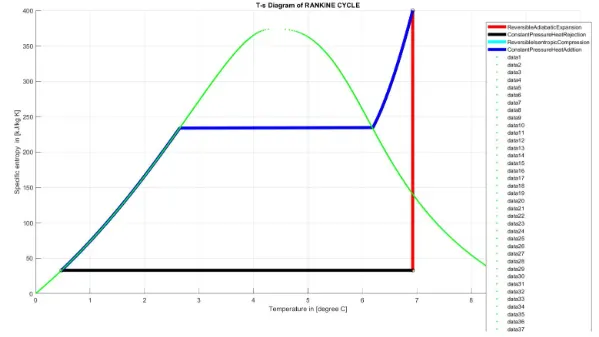
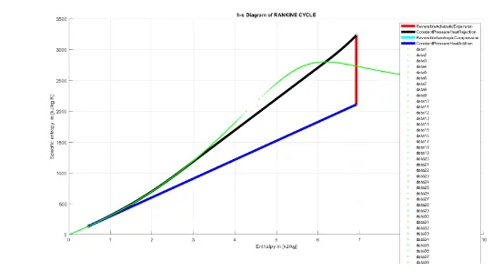
CONCLUSION :

• The state points of the Rankine Cycle are calculated by using the steam table data for water from standard MATLAB Xsteam library.

• Various programs to compute property values of water at three regions are developed using MATLAB. Those programs are then employed by another program which will simulate a Rankine cycle.

T-s, h-s and p-v plots of the Rankine Cycle are plotted and therefore the work and efficiency of the Rankine Cycle are calculated.