Project 2 - Rankine cycle Simulator

Course: MATLAB for Mechanical Engineers

Project 2: Rankine Cycle Simulator

Submitted By: Amanpreet Singh Whan

1 Aim:

The aim of the Project 2 challenge is to create a Rankine Cycle Simulator using MATLAB software.

2 Theory and Governing Equations:

The Rankine cycle or Rankine Vapor Cycle is the process widely used by power plants such as coal-fired power plants or nuclear reactors. In this mechanism, a fuel is used to produce heat within a boiler, converting water into steam which then expands through a turbine producing useful work. This process was developed in 1859 by Scottish engineer William J.M. Rankine. This thermodynamic cycle converts heat into mechanical energy, which is usually transformed into electricity by electrical generation.

The steps in the Rankine Cycle as shown in Figure 1 and the corresponding steps in the pressure-volume diagram (figure 2) are outlined below:

• Pump: Compression of the fluid to high pressure using a pump (this takes work)
• Boiler: The compressed fluid is heated to the final temperature (which is at boiling point), therefore, a phase change occurs—from liquid to vapor
• Turbine: Expansion of the vapor in the turbine
• Condenser: Condensation of the vapor in the condenser (where the waste heat goes to the final heat sink (the atmosphere or a large body of water (ex. lake or river).

The efficiency of the Rankine cycle is limited by the high heat of vaporization by the fluid. The fluid must be cycled through and reused constantly, therefore; water is the most practical fluid for this cycle. This is not why many power plants are located near a body of water—that's for the waste heat.

As the water condenses in the condenser, waste heat is given off in the form of water vapor—which can be seen billowing from a plant's cooling towers. This waste heat is necessary for any thermodynamic cycle. Due to this condensation step, the pressure at the turbine outlet is lowered. This means the pump requires less work to compress the water—resulting in higher overall efficiencies.

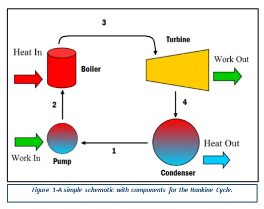
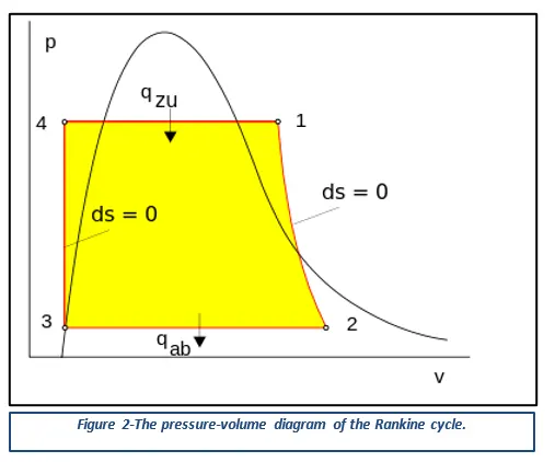
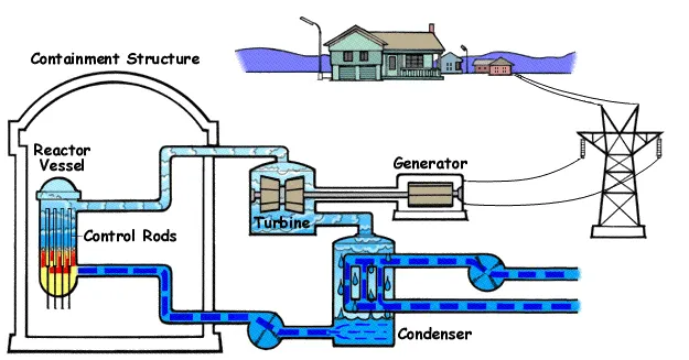
Figure 3- Rankine Cycle in a Nuclear Power Plant.

3 Objectives:

The objectives of the Project 2 challenges are as follows:

• Write a program that can perform the operation of the Rankine Cycle.
• The Program should calculate the state points of the Rankine Cycle based on user inputs.
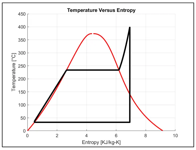
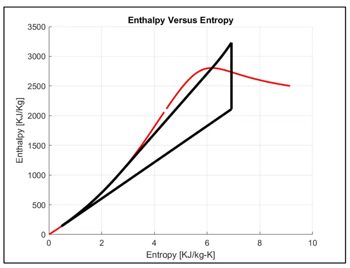
• Lastly, Plot the corresponding T-s and h-s plots for the given set of user inputs.

4 Body of the Content:

MATLAB (an abbreviation of "MATrix LABoratory") is a proprietary multi-paradigm programming language and numeric computing environment developed by MathWorks. MATLAB allows matrix manipulations, plotting of functions and data, implementation of algorithms, creation of user interfaces, and interfacing with programs written in other languages. Although MATLAB is intended primarily for numeric computing, an optional toolbox uses the MuPAD symbolic engine allowing access to symbolic computing abilities. An additional package, Simulink, adds graphical multi-domain simulation and model-based design for dynamic and embedded systems.

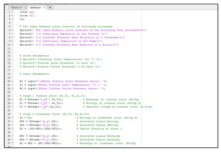
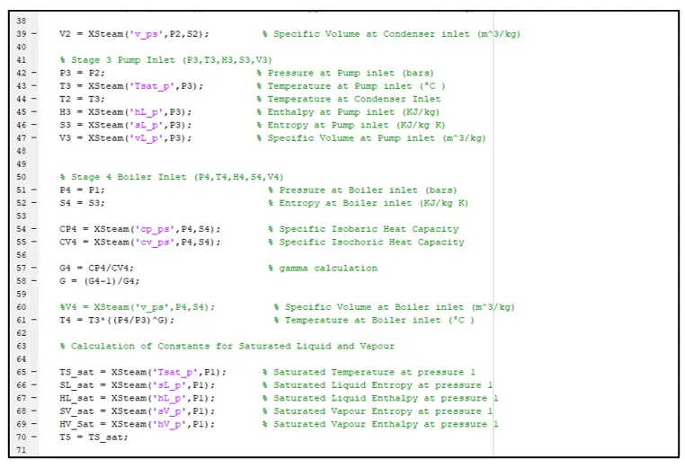
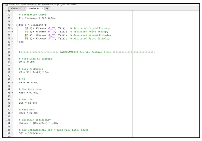
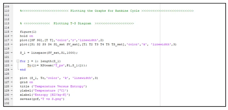
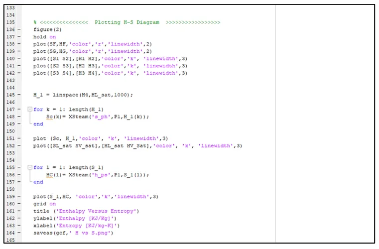
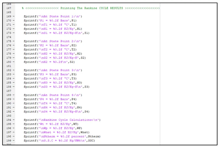
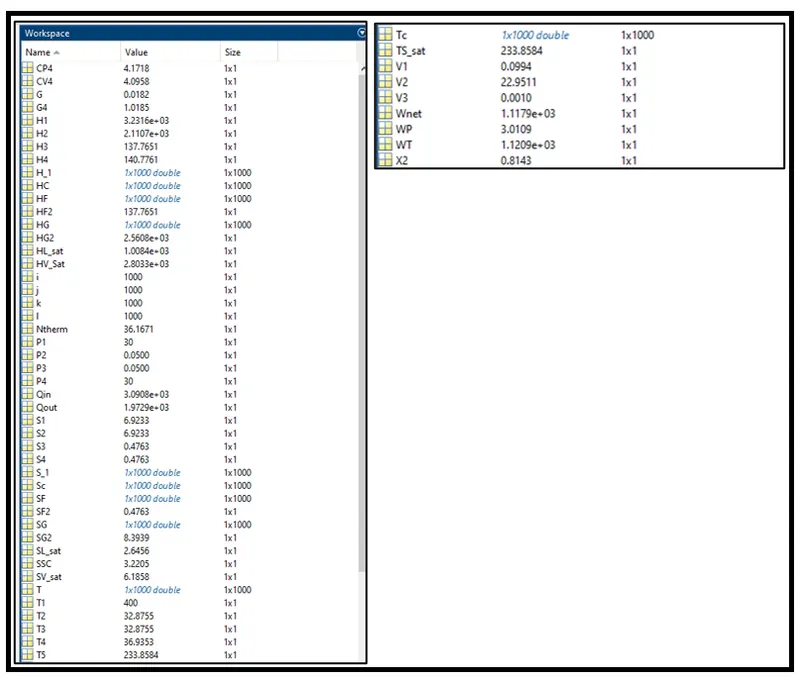
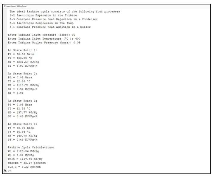
The code was written to fulfill the requirements of the Project 2 challenge and is attached in the following figures. In addition, the created plots from the written code are attached as well.

Rankine Cycle Simulator Code

Results

5 Conclusion:

In conclusion, the main aim of the Project 2 challenge is to create a Rankine Cycle Simulator using MATLAB that can Calculate its State Points and plot “Temperature versus Entropy” and “Enthalpy versus Entropy” graphs for user-defined inputs.

6 Appendix:

clear all
close all
clc

% The ideal Rankine cycle consists of following processes.
fprintf(' The ideal Rankine cycle consists of the following four processes\n')
fprintf(' 1-2 Isentropic Expansion in the Turbine \n') 
fprintf(' 2-3 Constant Pressure Heat Rejection in a Condenser\n')
fprintf(' 3-4 Isentropic Compresion in the Pump\n')
fprintf(' 4-1 Constant Pressure Heat Addition in a boiler\n')


% Given Parameters
% fprintf('\nTurbine Inlet Temperature: 400 °C \n')
% fprintf('Turbine Inlet Pressure: 30 bars \n')
% fprintf('Turbine Outlet Pressure: 0.05 bars \n')

% Input Parameters

P1 = input('\nEnter Turbine Inlet Pressure (bars): ');
T1 = input('Enter Turbine Inlet Temperature (°C ): ');
P2 = input('Enter Turbine Outlet Pressure (bars): ');

% Stage 1 Turbine Inlet (P1,T1, H1,S1,V1)
H1 = XSteam('h_pT', P1,T1);            % Enthalpy at turbine inlet (KJ/kg)
S1 = XSteam('s_pT', P1,T1);            % Entropy at turbine inlet (KJ/kg K)
V1 = XSteam('v_pT',P1,T1);             % Specific Volume at turbine inlet (m^3/kg)

% Stage 2 Condenser Inlet (P2,T2, H2,S2,V2)
S2 = S1;                           % Entropy at Condender inlet (KJ/kg K)
SF2 = XSteam('sL_p',P2);           % Saturated Liquid Entropy 
SG2 = XSteam('sV_p',P2);           % Saturated Vapour Entropy 
X2 = ((S2-SF2)/(SG2-SF2));         % Vapour Fraction at state 2

HF2 = XSteam('hL_p',P2);           % Saturated Liquid Enthalpy        
HG2 = XSteam('hV_p',P2);           % Saturated Vapour Enthalpy 
H2 = HF2 + (X2*(HG2-HF2));         % Enthalpy at Condenser inlet (KJ/kg)

V2 = XSteam('v_ps',P2,S2);         % Specific Volume at Condenser inlet (m^3/kg)

% Stage 3 Pump Inlet (P3,T3,H3,S3,V3)
P3 = P2;                          % Pressure at Pump inlet (bars)
T3 = XSteam('Tsat_p',P3);         % Temperature at Pump inlet (°C )
T2 = T3;                          % Temperature at Condenser Inlet
H3 = XSteam('hL_p',P3);           % Enthalpy at Pump inlet (KJ/kg)
S3 = XSteam('sL_p',P3);           % Entropy at Pump inlet (KJ/kg K)
V3 = XSteam('vL_p',P3);           % Specific Volume at Pump inlet (m^3/kg)


% Stage 4 Boiler Inlet (P4,T4,H4,S4,V4)
P4 = P1;                            % Pressure at Boiler inlet (bars)
S4 = S3;                            % Entropy at Boiler inlet (KJ/kg K)

CP4 = XSteam('cp_ps',P4,S4);        % Specific Isobaric Heat Capacity
CV4 = XSteam('cv_ps',P4,S4);        % Specific Isochoric Heat Capacity

G4 = CP4/CV4;                       % gamma calculation
G = (G4-1)/G4;

%V4 = XSteam('v_ps',P4,S4);          % Specific Volume at Boiler inlet (m^3/kg)
T4 = T3*((P4/P3)^G);                 % Temperature at Boiler inlet (°C )

% Calculation of Constants for Saturated Liquid and Vapour

TS_sat = XSteam('Tsat_p',P1);      % Saturated Temperature at pressure 1
SL_sat = XSteam('sL_p',P1);        % Saturated Liquid Entropy at pressure 1
HL_sat = XSteam('hL_p',P1);        % Saturated Liquid Enthalpy at pressure 1
SV_sat = XSteam('sV_p',P1);        % Saturated Vapour Entropy at pressure 1
HV_Sat = XSteam('hV_p',P1);        % Saturated Vapour Enthalpy at pressure 1
T5 = TS_sat;

% Saturation Curve
T = linspace(0,380,1000);

for i = 1:length(T)
    SF(i)= XSteam('sL_T', T(i));  % Saturated Liquid Entropy 
    SG(i)= XSteam('sV_T', T(i));  % Saturated Vapor Entropy 
    HF(i)= XSteam('hL_T', T(i));  % Saturated Liquid Enthalpy 
    HG(i)= XSteam('hV_T', T(i));  % Saturated Vapor Enthalpy 
end


%<<<<<<<<<<<<<<<<<<<<<<<<< CALCULATIONS for the Rankine Cycle >>>>>>>>>>>>>>>>>>>>>>>>>>>>

% Work Done by Turbine
WT = H1-H2;

% Work Performed
WP = V3*(P4-P3)*100;

% H4
H4 = WP + H3;

% Net Work done
Wnet = WT-WP;

% Heat in
Qin = H1-H4;

% Heat out
Qout = H2-H3;

% Thermal; Efficiency
Ntherm = (Wnet/Qin) * 100;

% SSC Consumption, SSc = mass flow rate/ power
SSC = 3600/Wnet;  


%<<<<<<<<<<<<<<<<<<<<<<<<< Plotting the Graphs for Rankine Cycle >>>>>>>>>>>>>>>>>>>>>>>>>>>>


% <<<<<<<<<<<<<<  Plotting T-S Diagram  >>>>>>>>>>>>>>>>>>>>>

figure(1)
hold on
plot([SF SG],[T T],'color','r','linewidth',2)
plot([S1 S2 S3 S4 SL_sat SV_sat],[T1 T2 T3 T4 T5 TS_sat],'color','k', 'linewidth',3)

S_1 = linspace(SV_sat,S1,1000);

for j = 1: length(S_1)
    Tc(j)= XSteam('T_ps',P1,S_1(j));
end

plot (S_1, Tc,'color', 'k', 'linewidth',3)
grid on
title ('Temperature Versus Entropy')
ylabel('Temperature [°C]')
xlabel('Entropy [KJ/kg-K]')
saveas(gcf,'T vs S.png')



% <<<<<<<<<<<<<<<  Plotting H-S Diagram  >>>>>>>>>>>>>>>>>
figure(2)
hold on
plot(SF,HF,'color','r','linewidth',2)
plot(SG,HG,'color','r','linewidth',2)
plot([S1 S2],[H1 H2],'color','k', 'linewidth',3)
plot([S2 S3],[H2 H3],'color','k', 'linewidth',3)
plot([S3 S4],[H3 H4],'color','k', 'linewidth',3)


H_1 = linspace(H4,HL_sat,1000);

for k = 1: length(H_1)
    Sc(k)= XSteam('s_ph',P1,H_1(k));
end

plot (Sc, H_1,'color', 'k', 'linewidth',3)
plot([SL_sat SV_sat],[HL_sat HV_Sat],'color', 'k', 'linewidth',3)


for l = 1: length(S_1)
    HC(l)= XSteam('h_ps',P1,S_1(l));
end

plot(S_1,HC, 'color','k','linewidth',3)
grid on
title ('Enthalpy Versus Entropy')
ylabel('Enthalpy [KJ/Kg]')
xlabel('Entropy [KJ/kg-K]')
saveas(gcf,' H vs S.png')


% <<<<<<<<<<<<<<<<<< Printing The Rankine CYCLE RESULTS >>>>>>>>>>>>>>>>>>>

 fprintf('\nAt State Point 1:\n')
 fprintf('P1 = %0.2f Bars',P1)
 fprintf('\nT1 = %0.2f °C',T1)
 fprintf('\nH1 = %0.2f KJ/Kg',H1)
 fprintf('\nS1 = %0.2f KJ/Kg-K\n',S1)
 
 fprintf('\nAt State Point 2:\n')
 fprintf('P2 = %0.2f Bars',P2)
 fprintf('\nT2 = %0.2f °C',T2)
 fprintf('\nH2 = %0.2f KJ/Kg',H2)
 fprintf('\nS2 = %0.2f KJ/Kg-K',S2)
 fprintf('\nX2 = %0.2f\n',S2)
 
 fprintf('\nAt State Point 3:\n')
 fprintf('P3 = %0.2f Bars',P3)
 fprintf('\nT3 = %0.2f °C',T3)
 fprintf('\nH3 = %0.2f KJ/Kg',H3)
 fprintf('\nS3 = %0.2f KJ/Kg-K\n',S3)
 
 fprintf('\nAt State Point 4:\n')
 fprintf('P4 = %0.2f Bars',P4)
 fprintf('\nT4 = %0.2f °C',T4)
 fprintf('\nH4 = %0.2f KJ/Kg',H4)
 fprintf('\nS4 = %0.2f KJ/Kg-K\n',S4)
 
 fprintf('\nRankine Cycle Calculations:\n')
 fprintf('Wt = %0.2f KJ/Kg',WT)
 fprintf('\nWp = %0.2f KJ/Kg',WP)
 fprintf('\nWnet = %0.2f KJ/Kg',Wnet)
 fprintf('\nNtherm = %0.2f percent',Ntherm)
 fprintf('\nS.S.C = %0.2f Kg/KWh\n',SSC)