CODE:
clear variables
close all
clc
disp(' RANKINE CYCLE SIMULATOR')
% Boiler outlet (Turbine Inlet)
disp('Process 1-2 isentropic expansion in turbine')
% Turbine Outlet (Condensor Inlet)
disp('Process 2-3 constant pressure heat rejection in condenser')
% Condensor Outlet (Pump Inlet)
disp('Process 3-4 Isentropic compression in pump')
% Pump Outlet (Boiler Inlet)
disp('Process 4-1 constant pressure heat addition by the boiler')
%State 1
%given
t1 = 400;
p1 = 30;
v1 = XSteam('v_pT', p1, t1);
s1 = XSteam('s_pT', p1, t1);
h1 = XSteam('h_pT', p1, t1);
%State 2
p2 = 0.05;
t2 = XSteam('Tsat_p', p2);
% Entropy of saturated liquid
sf = XSteam('sL_p', 0.05);
% Entropy change during evaporation
sfg = XSteam('sV_p', 0.05) - sf;
% Enthalpy of saturated liquid
hf = XSteam('hL_p', 0.05);
% Enthalpy change during evaporation
hfg = XSteam('hV_p', 0.05) - hf;
% Specific volume of saturated liquid
vf = XSteam('vL_p', 0.05);
% Volume change during evaporation
vfg = XSteam('vV_p', 0.05) - vf;
% quality
q2 = (s1-sf)/sfg;
s2 =s1;
h2 = hf + q2 * hfg;
v2 = vf + q2 * vfg;
% State 3
p3 = p2;
t3 = t2;
v3 = XSteam('vL_p', p3);
s3 = XSteam('sL_p', p3);
h3 = XSteam('hL_p', p3);
% State 4
p4 = p1;
s4 = s3;
%work done by pump
wp = v3 * (p4 - p3) * 100; %(kJ/kg)
%gamma = cp4/cv4
%cp4-cv4 =R
cp4 = XSteam('Cp_ps',p4,s4);
cv4 = XSteam('Cv_ps',p4,s4);
gamma = cp4/cv4;
r = (gamma-1)/gamma;
t4 = t3*((p4/p3)^r);
v4 = XSteam('vL_p', p4);
h4 = h3 + wp;
%state 5
t5 = XSteam('Tsat_p',p1);
h5 = XSteam('hL_p',p1);
s5 = XSteam('sL_p',p1);
% State 6
t6=t5;
h6 = XSteam('hV_p',p1);
s6 = XSteam('sV_p',p1);
%work done by turbine
wt = h1-h2;
%net work
wnet = wt-wp;
% heat transfer in boiler
qin = h1-h4;
% heat transfer in condenser
qout = h2-h3;
%Thermal efficiency
nthermal = (wnet/qin)*100;
%Back work ratio
BWR = wp/wt;
% T-s Diagram (Temperature vs. Entropy)
figure(1)
hold on;
axis([0 8 0 450])
plot(s1,t1,'*','color','r');
plot([s1 s2],[t1 t2],'LineWidth',2)
plot(s2,t2,'*','color','g');
plot([s2 s3],[t2 t3],'LineWidth',2)
plot(s3,t3,'*','color','b');
plot([s3 s4],[t3 t4],'LineWidth',2)
plot(s4,t4,'*','color','k');
plot([s4 s5],[t4 t5],'LineWidth',2)
plot(s5,t5,'*','color','y');
plot([s5 s6],[t5 t6],'LineWidth',2)
plot(s6,t6,'*','color','c');
plot([s6 s1],[t6 t1],'LineWidth',2)
text(s1,t1,'1','VerticalAlignment','bottom','HorizontalAlignment','left')
text(s2,t2,'2','VerticalAlignment','bottom','HorizontalAlignment','left')
text(s3,t3,'3','VerticalAlignment','top','HorizontalAlignment','right')
text(s4,t4,'4','VerticalAlignment','bottom','HorizontalAlignment','right')
text(s5,t5,'5','VerticalAlignment','bottom','HorizontalAlignment','left')
text(s6,t6,'6','VerticalAlignment','bottom','HorizontalAlignment','right')
xlabel('Entropy (kJ/kg·K)');
ylabel('Temperature (C)');
title('T-S Diagram');
grid on;
% H-s Diagram (Enthalpy vs. Entropy)
figure(2)
hold on;
axis([-1 8 -500 4000])
plot(s1,h1,'*','color','r');
plot([s1 s2],[h1 h2],'LineWidth',2)
plot(s2,h2,'*','color','g');
plot([s2 s3],[h2 h3],'LineWidth',2)
plot(s3,h3,'*','color','b');
plot([s3 s4],[h3 h4],'LineWidth',2)
plot(s4,h4,'*','color','k');
plot([s4 s1],[h4 h1],'LineWidth',2)
text(s1,h1,'1')
text(s2,h2,'2')
text(s3,h3,'3','VerticalAlignment','top')
text(s4,h4,'4','VerticalAlignment','bottom')
xlabel('Entropy (kJ/kg·K)');
ylabel('Enthalpy (kJ/kg)');
title('H-S Diagram');
grid on;
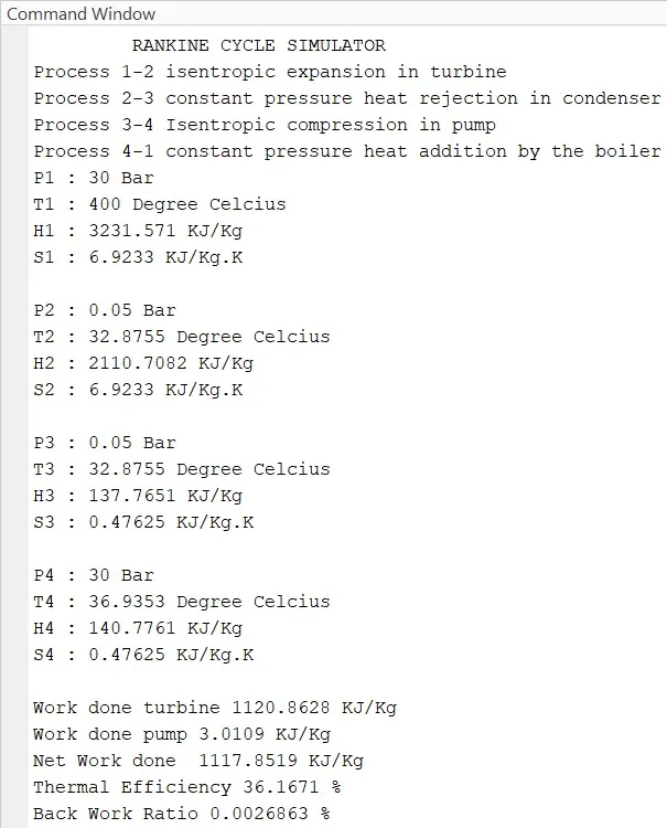
disp(['P1 : ' num2str(p1) ' Bar']);
disp(['T1 : ' num2str(t1) ' Degree Celcius']);
disp(['H1 : ' num2str(h1) ' KJ/Kg']);
disp(['S1 : ' num2str(s1) ' KJ/Kg.K']);
disp(' ')
disp(['P2 : ' num2str(p2) ' Bar']);
disp(['T2 : ' num2str(t2) ' Degree Celcius']);
disp(['H2 : ' num2str(h2) ' KJ/Kg']);
disp(['S2 : ' num2str(s2) ' KJ/Kg.K']);
disp(' ')
disp(['P3 : ' num2str(p3) ' Bar']);
disp(['T3 : ' num2str(t3) ' Degree Celcius']);
disp(['H3 : ' num2str(h3) ' KJ/Kg']);
disp(['S3 : ' num2str(s3) ' KJ/Kg.K']);
disp(' ')
disp(['P4 : ' num2str(p4) ' Bar']);
disp(['T4 : ' num2str(t4) ' Degree Celcius']);
disp(['H4 : ' num2str(h4) ' KJ/Kg']);
disp(['S4 : ' num2str(s4) ' KJ/Kg.K']);
disp(' ')
disp(['Work done turbine ' num2str(wt) ' KJ/Kg' ])
disp(['Work done pump ' num2str(wp) ' KJ/Kg' ])
disp(['Net Work done ' num2str(wnet) ' KJ/Kg' ])
disp(['Thermal Efficiency ' num2str(nthermal) ' %' ])
disp(['Back Work Ratio ' num2str(BWR) ' %' ])
OUTPUT:
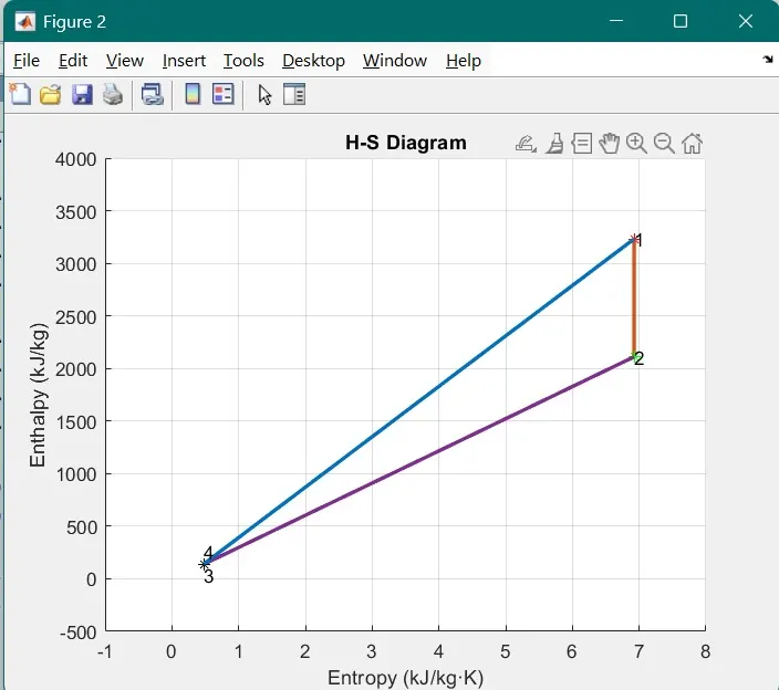
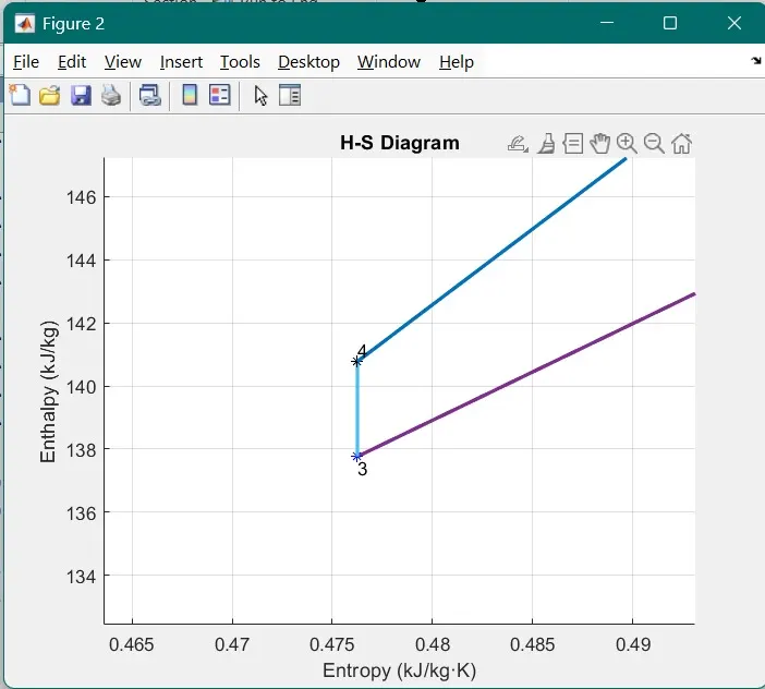
H-S diagram here points 3, 4 seems overlapping. but, when
zoomed can be seen separately as the values of them are too close
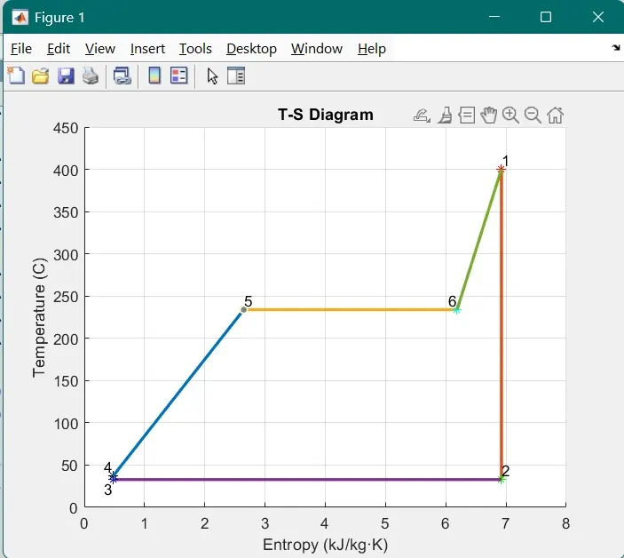
T-S diagram here points 3, 4 seems overlapping. but, when
zoomed can be seen separately as the values of them are too close
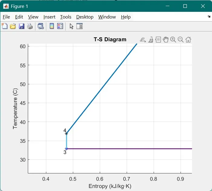
Rankine Cycle Simulator working:
=> In this cycle we basically have 4 states but including 2 substates due to superheating we have 6 states
* We already have temperature and pressure values of 1 stage further we also have another pressure value. rest of them should be found
* Here we have some of quantities are same for any of two stages lets discvuss them first.
>>s2 = s1; p3 = p2; t3 = t2; p4 = p1; s4 = s3; t6 = t5.
* These are values that are equal to respective stages because of their thermodynamic properties some value doesn't change from stage to stage
* For stage 2 volume and entropy we use the equation of properties for saturated liquid, and during evaporation.
* Stage 3 by the XSteam command of steam library.
* For stage 4 we use gamma equation to find t4 and h4 is sum of enthalpy during stage 3 and work done by pump.
* And the remaining by steam library.
* By now we get all the state values for all thermodynamic quantities required.
* We use those to plot the required T-S & H-S Diagrams.
**Coming to errors there were errors faced only for plotting as all the values are just mathematical relations of cycle. Encountering errors related to code were just the XSteam command realated which were not captured in the command window
**Research done include many videos from Youtube browsing through online pdf based on Rankine cycle and steam tables. Also, information related to XSteam is found in mathworks official website.
It also includes live sessions and videos from Skill Lync.