Project 2 - Rankine cycle Simulator
RANKINE CYCLE SIMULATION
AIM
Developing a Rankine cycle simulator in MATLAB, including the plotting of T-S and H-S diagrams based on the provided inputs.
INTRODUCTION
The Rankine cycle is a fundamental thermodynamic cycle used in thermal power plants to convert heat energy into mechanical work, which is later converted into electricity. This report details the creation of a program based on Rankine cycle, using the XSteam file for steam property calculations. The program computes state points, evaluates thermal efficiency and generates T-S and H-S plots to visualize the cycle.
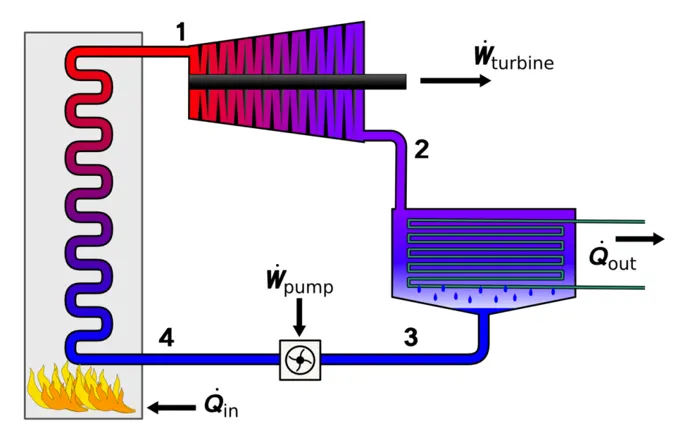
WORKING OF RANKINE CYCLE
Turbine (Expansion): High-pressure, high-temperature steam expands in the turbine, generating mechanical work. The steam’s pressure and temperature decrease during the process.
Condenser (Heat Rejection): The low-pressure steam exits the turbine and is cooled in the condenser, converting it into liquid by releasing heat.
Pump (Compression): The liquid is pressurized by a pump, preparing to reenter the boiler.
Boiler (Heat Addition): The high-pressure liquid absorbs heat in the boiler, converting into high pressure, high temperature steam.
Turbine Work (Wt) = h1 – h2
Pump Work (Wp) = h4 – h3
Heat Addition in Boiler (Qin) = h1 – h4
Heat Rejected in Condenser (Qout) = h2 – h3
Net Work Output (Wnet) = Wt – Wp
Thermal Efficiency (ɳ) = Wnet/Qin
Specific Steam Consumption (SSC) = 3600/Wnet
h1, h2, h3, h4 implies to enthalpy at each state point
STEP WISE EXPLANATION
Basic note about Rankine cycle is displayed.
disp('---Rankine Cycle Simulator---');
disp('Processes in the cycle :');
disp('1-2 : Isentropic expansion in turbine');
disp('2-3 : Constant pressure heat rejection in condenser');
disp('3-4 : Isentropic expansion in pump');
disp('4-1 : Constant pressure heat addition in boiler')
given inputs are added.
p1 = 30; % Pressure at turbine inlet
T1 = 400; % Temperature at turbine inlet
p2 = 0.5; % Pressure at condenser inlet
Thermodynamic data for each state points is either obtained from the XSteam file or calculated based on relevant equation. Additionally, efficiency and Specific Steam Consumption are also calculated.
% Collecting data from xsteam for each state point
% State 1 : Turbine inlet
h1 = XSteam('h_pT',p1,T1); % Enthalpy at p1 and t1
s1 = XSteam('s_pT',p1,T1); % Entropy at p1 and t1
% State 2 : Turbine outlet (Isentropic expansion)
s2 = s1; % 1-2 Isentropic process (Entropy constant)
sf2 = XSteam('sL_p',p2); % Saturated liquid entropy at p2
sg2 = XSteam('sV_p',p2); % Saturated vapour entropy at p2
x2 = (s2 - sf2)/(sg2 - sf2); % Vapour quality at state 2
hf2 = XSteam('hL_p',p2); % Saturated liquid enthalpy at p2
hg2 = XSteam('hV_p',p2); % Saturated vapour enthalpy at p2
h2 = hf2 + x2*(hg2 - hf2); % Enthalpy at state 2
T2 = XSteam('T_ps',p2,s2); % Temperature at state 2
% State 3 : Condenser outlet
p3 = p2; % 2-3 Constant pressure heat rejection in condenser
h3 = XSteam('hL_p',p3); % Saturated liquid enthalpy at p3
s3 = XSteam('sL_p',p3); % Saturated liquid entropy at p3
T3 = XSteam('Tsat_p',p3); % Saturation temperature at p3
% State 4 : Pump outlet (Isentropic compression)
s4 = s3; % 3-4 Isentropic process (Entropy constant)
p4 = p1; % 4-1 Constant pressure heat addition in boiler
v3 = XSteam('vL_p',p3); % Specific volume of liquid at p3
Wp = v3*(p4 - p3)*100; % Pump work done
h4 = h3 + Wp; % Enthalpy at state 4
T4 = XSteam('T_ph',p4,h4); % Temperature at state 4
% Rankine cycle effeciency calculation
Wt = h1 - h2; % Turbine work done
Wnet = Wt - Wp; % Net work done
Qin = h1 - h4; % Heat addition (Boiler)
Qout = h2 - h3; % Heat rejection (Condenser)
Eff = (Wnet/Qin)*100; % Thermal efficiency of rankine cycle
SCC = 3600/Wnet; % Specific steam consumption
% State 5 and State 6 data ( Pressure is constant)
T5 = XSteam('Tsat_p',p1);
s5 = XSteam('sL_p',p1);
h5 = XSteam('hL_p',p1);
T6 = T5;
s6 = XSteam('sV_p',p1);
h6 = XSteam('hV_p',p1);
Entropy and enthalpy for saturated liquid and saturated vapor are calculated for each temperature point to plot the saturation line.
T = linspace(1,560,1000);
for i = 1:length(T)
sf(i) = XSteam('sL_T',T(i)); % Saturated liquid entropy
sg(i) = XSteam('sV_T',T(i)); % Saturated vapour entropy
hf(i) = XSteam('hL_T',T(i)); % Saturated liquid enthalpy
hg(i) = XSteam('hV_T',T(i)); % Saturated vapour enthalpy
end
Additional calculations are done to get a better plot.
s_1 = linspace(s6,s1,1000);
for j = 1:length(s_1)
Tc(j) = XSteam('T_ps',p1,s_1(j));
end
hc = linspace(h4,h5,1000);
for k = 1:length(hc)
sc(k) = XSteam('s_ph',p1,hc(k));
end
for l = 1:length(s_1)
h_c(l) = XSteam('h_ps',p1,s_1(l));
end
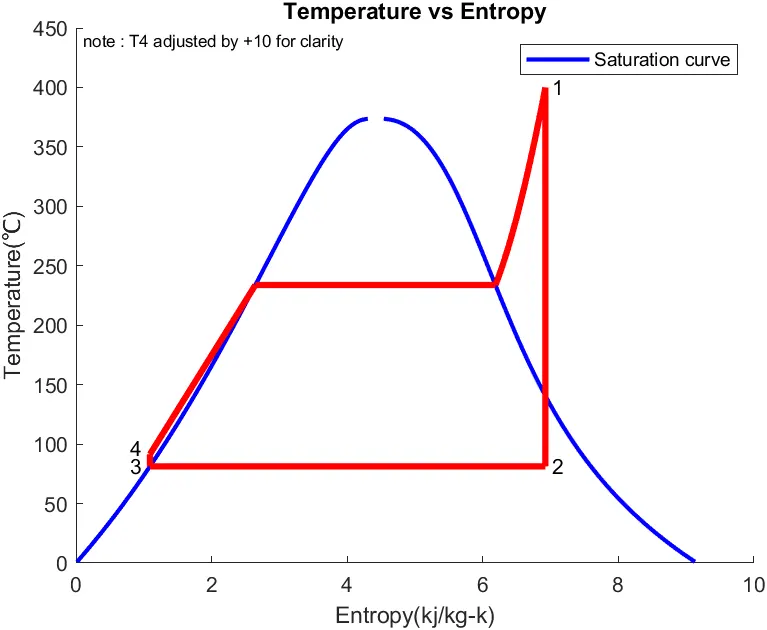
T-S and H-S diagram are plotted, In T-S diagram T4 is offset by + 10(T4_plot) for visualization due to the small temperature difference between T3 and T4.
% Plotting T-S Diagram
figure(1)
hold on
plot(sf, T,'Color','b','LineWidth',2)
plot(sg, T,'Color','b','LineWidth',2)
plot([s1 s2],[T1 T2],'Color','r','LineWidth',3)
plot([s2 s3],[T2 T3],'Color','r','LineWidth',3)
T4_plot = T4 + 10; % Because of negligible differenece between T3 and T4 for plot visualisation T4_plot is used instead of T4
plot([s3 s4],[T3 T4_plot],'Color','r','LineWidth',3)
plot([s4 s5],[T4_plot T5],'Color','r','LineWidth',3)
plot([s5 s6],[T5 T6],'Color','r','LineWidth',3)
plot(s_1,Tc,'Color','r','LineWidth',3)
text(s1+.1,T1,'1')
text(s2+.1,T2,'2')
text(s3-.3,T3,'3')
text(s4-.3,T4_plot+5,'4')
text(0.1,440,'note : T4 adjusted by +10 for clarity','FontSize',8)
ylim([0 450])
title('Temperature vs Entropy')
xlabel('Entropy(kj/kg-k)')
ylabel('Temperature(℃)')
legend('Saturation curve')
% Plotting H-S diagram
figure(2)
hold on
plot(sf, hf,'Color','b','LineWidth',2)
plot(sg, hg,'Color','b','LineWidth',2)
plot([s1 s2],[h1 h2],'Color','r','LineWidth',3)
plot([s2 s3],[h2 h3],'Color','r','LineWidth',3)
plot([s3 s4],[h3 h4],'Color','r','LineWidth',3)
plot(sc,hc,'Color','r','LineWidth',3)
plot([s5 s6],[h5 h6],'Color','r','LineWidth',3)
plot(s_1,h_c,'Color','r','LineWidth',3)
text(s1+.1,h1,'1')
text(s2+.1,h2,'2')
text(s3-.3,h3-150,'3')
text(s4-.3,h4+50,'4')
ylim([0 3600])
title('Enthalpy vs Entropy')
xlabel('Entropy(kj/kg-k)')
ylabel('Enthalpy(kj/kg)')
legend('Saturation curve')
To display the results in the command window.
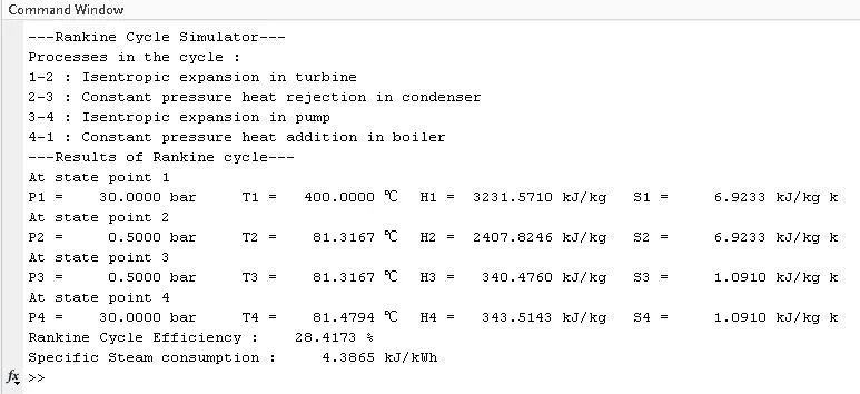
disp('---Results of Rankine cycle---')
fprintf('At state point 1\nP1 = %10.4f bar\t\tT1 = %10.4f ℃\tH1 = %10.4f kJ/kg\tS1 = %10.4f kJ/kg k\n',p1,T1,h1,s1)
fprintf('At state point 2\nP2 = %10.4f bar\t\tT2 = %10.4f ℃\tH2 = %10.4f kJ/kg\tS2 = %10.4f kJ/kg k\n',p2,T2,h2,s2)
fprintf('At state point 3\nP3 = %10.4f bar\t\tT3 = %10.4f ℃\tH3 = %10.4f kJ/kg\tS3 = %10.4f kJ/kg k\n',p3,T3,h3,s3)
fprintf('At state point 4\nP4 = %10.4f bar\t\tT4 = %10.4f ℃\tH4 = %10.4f kJ/kg\tS4 = %10.4f kJ/kg k\n',p4,T4,h4,s4)
fprintf('Rankine Cycle Efficiency : %10.4f %%\n',Eff)
fprintf('Specific Steam consumption : %10.4f kJ/kWh\n',SCC)
PROGRAM
close all
clear all
clc
% Rankine Cycle Simulation
% Display cycle information
disp('---Rankine Cycle Simulator---');
disp('Processes in the cycle :');
disp('1-2 : Isentropic expansion in turbine');
disp('2-3 : Constant pressure heat rejection in condenser');
disp('3-4 : Isentropic expansion in pump');
disp('4-1 : Constant pressure heat addition in boiler')
% Input data
p1 = 30; % Pressure at turbine inlet
T1 = 400; % Temperature at turbine inlet
p2 = 0.5; % Pressure at condenser inlet
% Collecting data from xsteam for each state point
% State 1 : Turbine inlet
h1 = XSteam('h_pT',p1,T1); % Enthalpy at p1 and t1
s1 = XSteam('s_pT',p1,T1); % Entropy at p1 and t1
% State 2 : Turbine outlet (Isentropic expansion)
s2 = s1; % 1-2 Isentropic process (Entropy constant)
sf2 = XSteam('sL_p',p2); % Saturated liquid entropy at p2
sg2 = XSteam('sV_p',p2); % Saturated vapour entropy at p2
x2 = (s2 - sf2)/(sg2 - sf2); % Vapour quality at state 2
hf2 = XSteam('hL_p',p2); % Saturated liquid enthalpy at p2
hg2 = XSteam('hV_p',p2); % Saturated vapour enthalpy at p2
h2 = hf2 + x2*(hg2 - hf2); % Enthalpy at state 2
T2 = XSteam('T_ps',p2,s2); % Temperature at state 2
% State 3 : Condenser outlet
p3 = p2; % 2-3 Constant pressure heat rejection in condenser
h3 = XSteam('hL_p',p3); % Saturated liquid enthalpy at p3
s3 = XSteam('sL_p',p3); % Saturated liquid entropy at p3
T3 = XSteam('Tsat_p',p3); % Saturation temperature at p3
% State 4 : Pump outlet (Isentropic compression)
s4 = s3; % 3-4 Isentropic process (Entropy constant)
p4 = p1; % 4-1 Constant pressure heat addition in boiler
v3 = XSteam('vL_p',p3); % Specific volume of liquid at p3
Wp = v3*(p4 - p3)*100; % Pump work done
h4 = h3 + Wp; % Enthalpy at state 4
T4 = XSteam('T_ph',p4,h4); % Temperature at state 4
% Rankine cycle effeciency calculation
Wt = h1 - h2; % Turbine work done
Wnet = Wt - Wp; % Net work done
Qin = h1 - h4; % Heat addition (Boiler)
Qout = h2 - h3; % Heat rejection (Condenser)
Eff = (Wnet/Qin)*100; % Thermal efficiency of rankine cycle
SCC = 3600/Wnet; % Specific steam consumption
% State 5 and State 6 data ( Pressure is constant)
T5 = XSteam('Tsat_p',p1);
s5 = XSteam('sL_p',p1);
h5 = XSteam('hL_p',p1);
T6 = T5;
s6 = XSteam('sV_p',p1);
h6 = XSteam('hV_p',p1);
% Plotting for saturation line
T = linspace(1,560,1000);
for i = 1:length(T)
sf(i) = XSteam('sL_T',T(i)); % Saturated liquid entropy
sg(i) = XSteam('sV_T',T(i)); % Saturated vapour entropy
hf(i) = XSteam('hL_T',T(i)); % Saturated liquid enthalpy
hg(i) = XSteam('hV_T',T(i)); % Saturated vapour enthalpy
end
% Intermediate calculation for turbine expansion
s_1 = linspace(s6,s1,1000);
for j = 1:length(s_1)
Tc(j) = XSteam('T_ps',p1,s_1(j));
end
hc = linspace(h4,h5,1000);
for k = 1:length(hc)
sc(k) = XSteam('s_ph',p1,hc(k));
end
for l = 1:length(s_1)
h_c(l) = XSteam('h_ps',p1,s_1(l));
end
% Plotting T-S Diagram
figure(1)
hold on
plot(sf, T,'Color','b','LineWidth',2)
plot(sg, T,'Color','b','LineWidth',2)
plot([s1 s2],[T1 T2],'Color','r','LineWidth',3)
plot([s2 s3],[T2 T3],'Color','r','LineWidth',3)
T4_plot = T4 + 10; % Because of negligible differenece between T3 and T4 for plot visualisation T4_plot is used instead of T4
plot([s3 s4],[T3 T4_plot],'Color','r','LineWidth',3)
plot([s4 s5],[T4_plot T5],'Color','r','LineWidth',3)
plot([s5 s6],[T5 T6],'Color','r','LineWidth',3)
plot(s_1,Tc,'Color','r','LineWidth',3)
text(s1+.1,T1,'1')
text(s2+.1,T2,'2')
text(s3-.3,T3,'3')
text(s4-.3,T4_plot+5,'4')
text(0.1,440,'note : T4 adjusted by +10 for clarity','FontSize',8)
ylim([0 450])
title('Temperature vs Entropy')
xlabel('Entropy(kj/kg-k)')
ylabel('Temperature(℃)')
legend('Saturation curve')
% Plotting H-S diagram
figure(2)
hold on
plot(sf, hf,'Color','b','LineWidth',2)
plot(sg, hg,'Color','b','LineWidth',2)
plot([s1 s2],[h1 h2],'Color','r','LineWidth',3)
plot([s2 s3],[h2 h3],'Color','r','LineWidth',3)
plot([s3 s4],[h3 h4],'Color','r','LineWidth',3)
plot(sc,hc,'Color','r','LineWidth',3)
plot([s5 s6],[h5 h6],'Color','r','LineWidth',3)
plot(s_1,h_c,'Color','r','LineWidth',3)
text(s1+.1,h1,'1')
text(s2+.1,h2,'2')
text(s3-.3,h3-150,'3')
text(s4-.3,h4+50,'4')
ylim([0 3600])
title('Enthalpy vs Entropy')
xlabel('Entropy(kj/kg-k)')
ylabel('Enthalpy(kj/kg)')
legend('Saturation curve')
% Displaying the results
disp('---Results of Rankine cycle---')
fprintf('At state point 1\nP1 = %10.4f bar\t\tT1 = %10.4f ℃\tH1 = %10.4f kJ/kg\tS1 = %10.4f kJ/kg k\n',p1,T1,h1,s1)
fprintf('At state point 2\nP2 = %10.4f bar\t\tT2 = %10.4f ℃\tH2 = %10.4f kJ/kg\tS2 = %10.4f kJ/kg k\n',p2,T2,h2,s2)
fprintf('At state point 3\nP3 = %10.4f bar\t\tT3 = %10.4f ℃\tH3 = %10.4f kJ/kg\tS3 = %10.4f kJ/kg k\n',p3,T3,h3,s3)
fprintf('At state point 4\nP4 = %10.4f bar\t\tT4 = %10.4f ℃\tH4 = %10.4f kJ/kg\tS4 = %10.4f kJ/kg k\n',p4,T4,h4,s4)
fprintf('Rankine Cycle Efficiency : %10.4f %%\n',Eff)
fprintf('Specific Steam consumption : %10.4f kJ/kWh\n',SCC)
RESULTS
Command window screen shot
T-S diagram
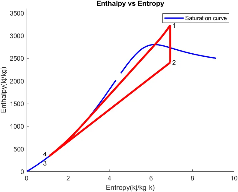
H-S diagram
CONCLUSION
The Rankine cycle simulator calculates thermodynamic properties at each state point and evaluates key performance metrics. The T-S and H-S plots provides a clear visualization of the cycle.