Project 2 - Rankine cycle Simulator
RANKINE CYCLE SIMULATOR
AIM: Create a Rankine CycleSimulator using OCTAVE/MATLAB.
OBJECTIVE:
- Create a Rankine Cycle using OCTAVE/MATLAB.
- Yourcode should calculate the state points of the Rankine Cycle (any type of choice) based on user input.
- Then plot the corresponding T-s and h-s plots for the given set of inputs. Title and axes labels are a must , while legends could be used if necessary.
- The presentation of your code will be taken into consideration while grading. labeling section of your code using comments is appreciated.
Attached a report explaining the working of a rankine cycle simulator and also the research was done by you.
Theory:
The Rankine Cycle is a model used to predict the performance of steam turbine system. It was also used to study the performance of reciprocating steam engines. The Rankine cycle is an idealized thermodynamic cycle in which engine that convert heat into mechanical work while undergoing a phase change.It is an idealized cycle in which friction losses in each of four components are neglected. The heat is supplied externally to aclosed loop, which usually uses water as the working fluid.
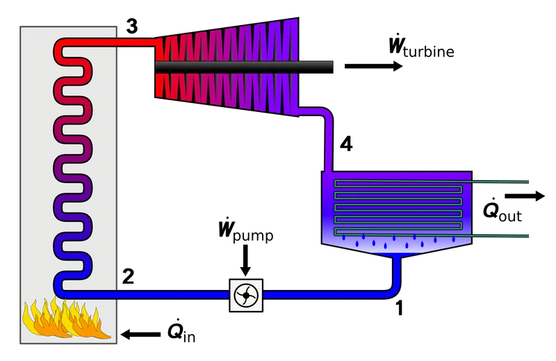
There are four processes in the rankine cycle. The states are identified by the numbers in T-s diagram.
- Process 1-2: The working fluid is pumped from low to high pressure. As the fluid is a liquid at this stage, the pump requires little input energy. In other words it is called isentropic compression.
- Process 2-3: The high pressure liquid enters a boiler , where it is heated at constant pressure by an external heat source to become a dry saturated vapor. The input energy required can be easily calculated graphically, using an enthalpy-entropy chat(h-s, or mollier diadram), or numerically, using the steam table. and the other name is constant pressure heat addition.
- Process 3-4: The dry saturated vapor expands through a turbine, genrating power. This decrease the temperatur and pressure of the vapor, and some condensation may occur. The output in this process can be easily calculated using the chart or tables noted above. and process called Isentropic expansion.
- Process4-1: The wet vapor then enters a condenser, whre it is condensed at a constant pressure to become a saturated liquid. and the words process is constant pressure heat rejection in condenser.
Explanation of code:
- We start the program by reading about the Rankine cycle and the given data and xsteam.
- First we need input data of pressure at the turbine inlet, the temperature at the turbine inlet, the pressure at condenser inlets.
- now we return the pressure and the temperature , by using the above- given data and xsteam.
- With this , we further simplify using the same data and the study over the rankine cycle.
- By all the study we calculate saturated liquid and saturated vapor through the plots.
- Then we calculate the total work , work done on the turbine, and the work done on the pump.
- We also calculate the efficiency and the spacific steam consumption.
- After the 4th stage of variation, we observe the plot by extracting the temperature enthalpy and entropy.
- Plotting graps of temerature vs enthalpy and enthalpy vs entropy while giving them line color and linewidth.
- As the input changes graph change.
- And the result will be displayed on the command window.
Programs code:
Input parameters

Turbine Inlet temperature = 400°c

Turbine Inlet pressure = 30 bars

turbine outlet pressure = 0.05 bars = condenser Inlet pressure

% A program for simulating Rankine cycle and plot required graphs.

closs all

clear all

clc

%subscript for different state points

%  1 = Turbine inlet or boiler outlet, 2 = condenser inlet or Turbine outlet,

% 3 = pump inlet or condenser outlet, 4 = Boiler inlet or pump outlet

%Inputs parameters

% p1 = Turbine inlet pressure(bar),

% t1 = Temperature at turbine inlet (deg c),

%p2 = Turbine outlet pressure (bar),

%Description about four process,

fprintf('process (1-2) - Isentropic expansion in the turbinen')

fprintf('process (2-3) - Isobaric heat rejection by the condensern')

fprintf('process (3-4) - Isentropic compression in the pumpn')

fprintf('process( (4-1) - Isobaric heat addition by the boilern')

%For inputting state variables at point 1,

p1 = input('Enter the pressure at the Turbine Inlet (in bar): ');

t1 = input('Enter the Temperature at the Turbine Inlet (in degree celcius): ');

p2 = input('Enter the pressure at the Turbine outlet ( in bar); ');

% State varible at state point 1,

h1 = Xsteam('h_pT' ,p1, t1);%Enthalpy in [kj/kg];

 s1 = Xsteam('s_pT' ,p1,t1);%specific entropy in [kj/kgk];

v1 = Xsteam('v_pT' ,p1, t1);%specific volume in [m^3/kg\];

% State variable at state point 2(i.e condenser Inlet)

s2 = s1;%specific entropy in [kj/kg k]

h2 = Xsteam('h_px' ,p2,Xsteam('x_ps' ,p2,s2));%Enthalpy in [kj/kg]

t2 = Xsteam('T_ps' , p2,s2);%Temperature in [degree celcious]

 v2 = Xsteam('v_ps' ,p2, s2);%specific volume in [m^3/kg]

%State variable at state point 3(i.e pump Inlet)

p3 = p2;%pressure in [bar]

t3 = Xsteam('Tsat_p' ,p3);%Temperature in [degree c]

h3 = Xteam('hL_p' ,p3);%enthalpy in [kj/kg]

s3 = Xsteam('sL_p' ,p3);%Specific Entropy in [kj/kg k]

v3 = Xsteam('vL_p' ,p3);%Inlet specific volume in [m^3/kg]

%State variable at point 4(i.e Boiler Inlet)

s4 = s3;%Specific entropy in [kj/kg k]

p4 = p1;%pressure in [bar]

h4 = Xsteam('h_ps' ,p4,s4);%Enthalpy in [kj/kg]

t4 = Xsteam('T_ps' ,p4 s4);%Temperature in [degree c]

v4 = Xsteam('v_ps' ,p4,s4);%specific volume in [m^3/kg]

% After defining all the states now lets process each of these state and in between data varibles

%Plotting Graph for Ideal Rankine cycle in "T" vs "s".

figure(1)

hold on

plot([s1 s2],[t1 t2], 'color' ,'r' ,'linewidth' ,5);

plot([s2 s3],[t2 t3], 'color' ,'k' ,'linewidth' ,5);

plot([s3 s4],[t3 t4], 'color' ,'c' ,'linewidth' ,5);

Trange = linespace(t4,t1,500);

for i = 1:length(Trange);

s_range(i) = Xsteam('s_pT' ,p1,Trange(i));

h_range23(i) = Xsteam('h_ps' ,p1,s_range(i));

h_range41(i) = Xsteam('h_ps' ,p2,s_range(i));

end

plot(s_range,Trange, 'color' ,'b' ,'linewidth' ,5);

legend('ReversibleadiabaticExpansion' , 'ConstantoressureheatRejecton' , 'ReversibleIsentropicCompression' , 'constantPressureheataddition');

%plotting Grapf for Ideal Rankine cycle in 'h' vs 's'.

figure(2)

hold on

plot([s1 s2],[h1 h2],'color' , 'r' , 'linewidth',5);

plot(s_range,h_range23,'color','k','linewidth',5);

plot([s3 s4],[h3 h4],'color' , 'c' , 'linewidth',5);

plot(s_range,h_range41,'color','b','linewidth',5);legend('ReversibleadiabaticExpansion' , 'ConstantoressureheatRejecton' , 'ReversibleIsentropicCompression' , 'constantPressureheataddition');

%ploting graphs for 'T' vs 's'

t_range = linespace(0,374.15,500);%Teperature from 0 to crtical point of water in [degree c]

figure(1)

hold on

for i  = 1:length(t_range);

plot(Xsteam('sL_t',t_range(i)),t_range(i),'.','color','g')

plot(Xsteam('sv_t',t_range(i)),t_range(i),'.','color','g')

end

%ploting graphs for 'T' vs 's'

figure()

hold on

for i  = 1:length(t_range);

plot(Xsteam('sL_t',t_range(i)),Xsteam('hL_t',t_range(i)),'.','color','g')

plot(Xsteam('sv_t',t_range(i)),Xsteam('hV_t',t_range(i)),'.','color','g')

end

%plotting Diagram for all state points for Ideal Rankine cycle in 'T' vs 's'

figure(1)

hold on

plot(s1,t1,'ko')

plot(s2,t2,'ko')

plot(s3,t3,'ko')

plot(s4,t4,'ko')

grid on

title('T_s Diagram of Rankine Cycle')

Xlabel('Temperature in [degree c]')

Ylabel('Specific entropy in [kj/kg k]')

%plotting Diagram for all state points for Ideal Rankine cycle in 'h' vs 's'

figure(2)

hold on

plot(s1,h1,'ko')

plot(s2,h2,'ko')

plot(s3,h3,'ko')

plot(s4,h4,'ko')

grid on

title('h_s Diagram of Rankine Cycle')

Xlabel('Enthalpy i n [kj/kg]')

Ylabel('Specific entropy in [kj/kg k]')

%Finally calulating work and Efficiency

work_turbine = h1- h2;%work transferred from the working fluid (kj/kg)

Q_taken_out_condenser = h2-h3;%heat rejected from working fluid(kj/kg)

work_pump = h4-h3;%work transferred into the working fluid (kj/kg)

Q_given_boiler = h1-h4;%heat transferred to the working fluid(kj/kg)

Back_work_ratio = work_turbine/work_pump;%Back work  Ratio

SSE = 3600/(work_turbine-work_pump);%specific Steam Consumption  [kg/kwh]

work_net = work_turbine-work_pump;%Net work on working fluid(kj/kg)

Effi_rankine = work_net/Q_given_boiler;%Rankine Cycle Efficiency

clc

%Printing Results to the user giving input

fprintf('Rankine Cycle:Ideal Cycle for vapour power Cyclenn');

fprintf('process 1-2: Reversible adiabatic expansion process in the  steam turbinen')

fprintf('process 2-3 :cosntant pressure  heat transfer in  the condensern')

fprintf('process 3-4: Reversible adiabatic compression process in the pumpn')

fprintf('process 4-1: constant pressure heat transfer process in the boilern')

fprintf('------State variable at state point 1-----n');

fprintf('Turbine Inlet Temperature T1 =%.5f in [degree c]n',t1);

fprintf('Turbine Inlet pressure p1 =%.5f in [bar]n',p1);

fprintf('Turbine Inlet Specific enthalpy h1 =%.5f in [kj/kg]n',h1);

fprintf('Turbine Inlet Specific entropy s1 =%.5f in [kj/kg k]n',s1);

fprintf('Turbine Inlet Specific volume v1 =%.5f in [m^3/kg]nn',v1);


fprintf('-----State variable at state point 2-----n');

fprintf('Condenser Inlet Temperature T1 =%.3f in [degree c]n',t2);

fprintf('Condenser Inlet pressure p1 =%.3f in [bar]n',p2);

fprintf('Condenser Inlet Specific enthalpy h1 =%.3f in [kj/kg]n',h2);

fprintf('Condenser Inlet Specific entropy h1 =%.3f in [kj/kg]n',s2);

fprintf('Condenser Inlet Specific volume v1 =%.3f in [m^3/kg]nn',v2);


fprintf('-----State variable at state point 3-------n');

fprintf('pump Inlet Temperature T1 =%.3f in [degree c]n',t3);

fprintf('pump Inlet pressure p1 =%.3f in [bar]n',p3);

fprintf('pump Inlet Specific enthalpy h1 =%.3f in [kj/kg]n',h3);

fprintf('pump Inlet Specific entropy h1 =%.3f in [kj/kg]n',s3);

fprintf('pump Inlet Specific volume v1 =%.3f in [m^3/kg]nn',v3);


fprintf('-----State variable at state point 4-------n');

fprintf('Boiler Inlet Temperature T1 =%.4f in [degree c]n',t4);

fprintf('Boiler Inlet pressure p1 =%.4f in [bar]n',p4);

fprintf('Boiler Inlet Specific enthalpy h1 =%.4f in [kj/kg]n',h4);

fprintf('Boiler Inlet Specific entropy h1 =%.4f in [kj/kg]n',s4);

fprintf('Boiler Inlet Specific volume v1 =%.4f in [m^3/kg]nn',v4);

fprintf('----work and Efficiency-----n');

fprintf('work transferred from working fluid wturbine =%.4f in [kj/kg]n',work_turbine);

fprintf('heat rejected from the vworking fluid Qcondenser = %.4f in [kj/kg]n',Q_taken_out_condenser);

fprintf('work transferred into the working fluid wpump = %.4f in [kj/kg]n',work_pump);

fprintf('heat transferred  to the vworking fluid Qboiler = %.4f in [kj/kg]n',Q_given_boiler);

fprintfd('Back work Ratio BWR = %.4f n',Back_work_Ratio);

fprintf('Specifc Steam Consumption SSE = %.4f in [kg/kwh]n', SSE);

fprintf('Net work on the working fluid wnet = %.4f in [kj/kg]n',work_net);
RESULT
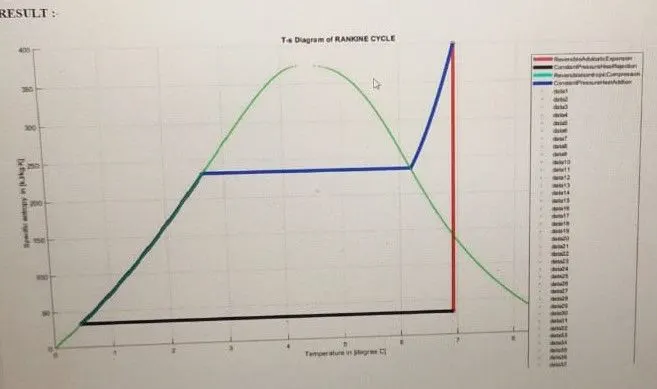
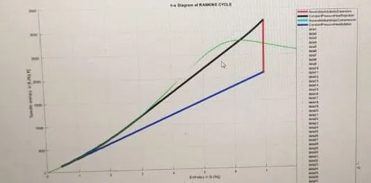
Process 1-2:Reversible adiabatic expansion process in the steam turbine
Process 2-3:Constant pressure heat transfer process in the condenser
Propcess 3-4:Reversible adiabatic compression process in the pump
Process 4-1:Constant pressure heat transfer in the boiler
-------State variable at state point 1---
Turbine Inlet Temperature T1 = 400.00000 in [degree c]
Turbine Inlet pressure p1 = 30.00000 in [bar]
Turbine Inlet Enthalpy h1 = 3231.57103 in [kj/kg ]
Turbine Inlet Specifi Entropy s1 = 6.92326 in [kj/kg k]
Turbine Inlet Specific volume v1 = 0.09938 in [m^3/kg]
-------State variable at state point 2---
Condenser Inlet Temperature T1 = 32.875 in [degree c]
Condenser Inlet pressure p1 = 0.050 in [bar]
Condenser Inlet Enthalpy h1 = 2110.708 in [kj/kg ]
Condenser Inlet Specifi Entropy s1 = 6.923 in [kj/kg k]
CondenserInlet Specific volume v1 = 22.95 in [m^3/kg]
-------State variable at state point3---
PumpInlet Temperature T1 = 32.875 in [degree c]
Pump Inlet pressure p1 = 0.050 in [bar]
Pump Inlet Enthalpy h1 = 137.765 in [kj/kg ]
Pump Inlet Specifi Entropy s1 = 0.476 in [kj/kg k]
PumpInlet Specific volume v1 = 0.001 in [m^3/kg]
-------State variable at state point3---
Boiler Inlet Temperature T1 = 32.9452 in [degree c]
Boiler Inlet pressure p1 = 30.0000 in [bar]
Boiler Inlet Enthalpy h1 = 140.7622 in [kj/kg ]
Boiler Inlet Specifi Entropy s1 = 0.4763 in [kj/kg k]
Boiler Inlet Specific volume v1 = 0.0010 in [m^3/kg]
-------work and Efficiency-----
work transferred from the working fluid wturbine = 1120.8628 in [kj/kg]
Heat rejected from the working fluid Qcondenser = 1972.9431 in [kj/kg]
work transferred into the working fluid wpump = 2.9971 in [kj/kg]
Heat transferred to the working fluid Qboiler = 3090.8088[kj/kg]
Back Work Ratio BWR = 373.9816
Specific Steam Consumption SSE = 3.2204 in [kg/kwh]
Net work on the working fluid Wnet = 1117.8657[kj/kg]
Rankine cycle Efficiency ETArankine = 36.1674%
-------- SUCESSFULLY DONE THE CALCULATIONS-------