Project 2 - Rankine cycle Simulator
Aim :
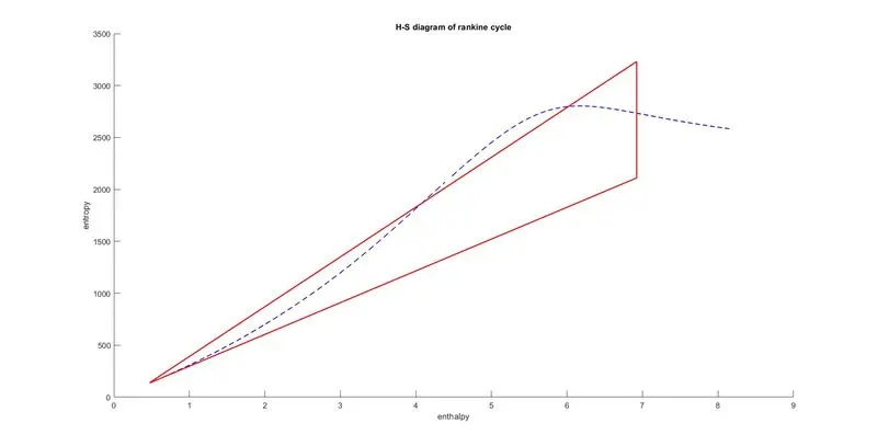
To create a Rankine cycle simulator using matlab, which should calculate state points using user inputs. and to create T-S and H-S plots for corresponding inputs.
Required Inputs:
Turbine Inlet temperature = 400° C
Turbine Inlet Pressure = 30 bars
Turbine Outlet Pressure = 0.05 bars = Condenser Inlet Pressure
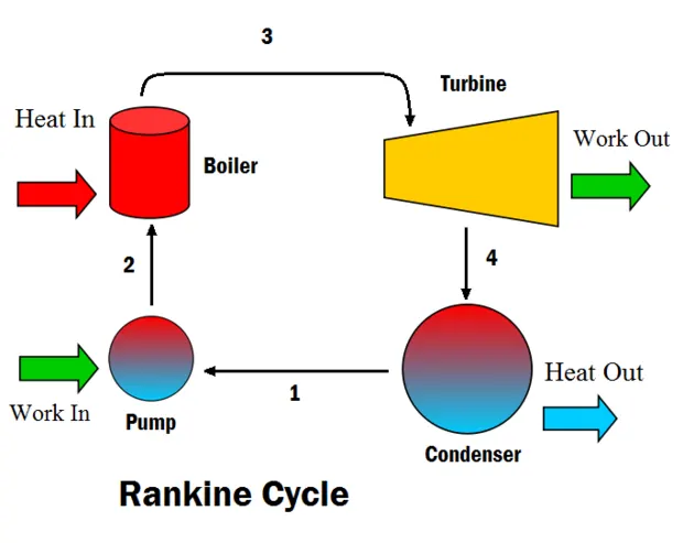
RANKINE CYCLE :
MATLAB CODE :
clear all
close all
clc

%print heading
fprintf('n                        RANKINE CYCLE SIMULATOR');
fprintf('nn1-2 is isentropic expansion in the turbine');
fprintf('n2-3 is constant pressure heat rejection by the condensor');
fprintf('n3-4 is isentropic compression in the pump');
fprintf('n4-1 is constant pressure heat addiction by the boiler');

%user input
p1 = input('nenter the pressure at the turbine inlet(in bar):');
t1 = input('enter the temperature at the turbine inlet(in degree celsius):');
p2 = input('enter the pressure at the condenser(in bar):');

%calculating various parameter for rankine cycle
%h - enthalpy
%s - entropy
%t - temperature
%p - pressure
%v - volume

%for state point 1
h1 = XSteam('h_pT',p1,t1);
s1 = XSteam('s_pT',p1,t1);

%for statepoint 3
p3 = p2;
h3 = XSteam ('hL_p',p3);
s3 = XSteam('sL_p',p3);
v3 = XSteam('vL_p',p3);
t3 = XSteam('Tsat_p',p3);

%for state point 2
t2 = t3;
s2 = s1;
sf2 = XSteam('sL_p',p2);
sg2 = XSteam('sV_p',p2);
hf2 = XSteam('hL_p',p2);
hg2 = XSteam('hV_p',p2);
x2 = ((s2-sf2)/(sg2-sf2));
h2 = hf2+(x2*(hg2-hf2));

%for state point 4
p4 = p1;
s4 = s3;
cp4 = XSteam('Cp_ps',p4,s4);
cv4 = XSteam('Cv_Ps',p4,s4);
g4 = cp4/cv4;
o = (g4-1)/g4;
t4 = t3*((p4/p3)^o);

%pump work
Wp = v3*(p4-p3)*100;

%wp = h4/h3 from this equation
h4 = h3+Wp;

%turbine work
Wt = h1-h2;

%network
Wnet = Wt-Wp;

%heat addiction at steam generator
Qin = h1-h4;

%heat rejection at condenser
Qout = h2-h4;

%thermal efficiency of cycle
Ntherm = (Wnet/Qin)*100;

%back work ratio : ratio of pump work required and turbine work generated
BWR = Wp/Wt;

%calculating values of liquid and vapour saturated lines

pressure_range = 0:0.1:400;

for i=1:length(pressure_range)
    tL_sat(i) = XSteam('Tsat_p',pressure_range(i));
    sL_sat(i) = XSteam('sL_p', pressure_range(i));
    sV_sat(i) = XSteam('sV_p', pressure_range(i));
    hL_sat(i) = XSteam('hL_p', pressure_range(i));
    hV_sat(i) = XSteam('hV_p', pressure_range(i));
end

%for plot from state 4 to 1 on T-S diagram different values

tp=XSteam('Tsat_p',p4);
s4_L=XSteam('sL_T',tp);
s4_V = XSteam('sV_T',tp);
t_range = linspace(tp, t1, 200);
for i=1:length(t_range)
    s4V_1(i) = XSteam('s_pT',p4,t_range(i));
end

%plot the results
%figure(1)-complete result
%figure(2)-enthalpy/entropy diagram
%figure(3)-temp vs entropy diagram

%define figure properties
figure('units','normalized','outerposition',[0 0 1 1])
figure(1)

%complete results using subplot
%plot heading and process name using subplot
ax = subplot(6,4,[1,2,3,4,5,6,7,8]);
text(0.4,1,'rankine cycle simulator','fontsize',12,'FontWeight','bold');
text(0,0.8,'1-2 is isentropic expansion in the turbine');
text(0,0.7,'2-3 is constant pressure heat rejection by the condensor');
text(0,0.6,'3-4 is isentropic compression in the pump');
text(0,0.5,'4-1 is constant pressure heat addition by the boiler');
text(0,0.3,['enter the pressure at the turbine inlet(in bar):',num2str(p1)]);
text(0,0.2,['enter the tem[erature at the turbine inlet(in degree celsius):',num2str(t1)]);
text(0,0.1,['enter the pressure at the condenser(in bar):',num2str(p2)]);
text(0.47,0,'result','FontWeight','bold');
set(ax,'visible','off')

%print stage 1 values
ax=subplot(6,4,[9,13]);
text(0,1,'at state point 1 : ');
text(0,0.8,['p1 is : ',num2str(p1),'bar']);
text(0,0.7,['t1 is : ',num2str(t1),'deg celsius']);
text(0,0.6,['h1 is :',num2str(h1),'kj/kg']);
text(0,0.5,['s1 is :',num2str(s1),'kj/kgk']);
set(ax,'visible','off')

%print work done and efficiency
text(0,0.3,'other results :');
text(0,0.2,['Wt is :',num2str(Wt),'kj/kg']);
text(0,0.1,['Wp is :',num2str(Wp),'kj/kg']);
text(0,0,['Wnet is :',num2str(Wnet),'kj/kg']);
set(ax,'visible','off')

%print stage 2 values
ax = subplot(6,4,[10,14]);
text(0,1,'at state point 2 :');
text(0,0.8,['p2 is :',num2str(p2),'bar']);
text(0,0.7,['t2 is :',num2str(t2),'deg celcius']);
text(0,0.6,['h2 is :',num2str(h2),'kj/kg']);
text(0,0.5,['s2 is :',num2str(s2),'kj/kgk']);
text(0,0.2,['BWR is :',num2str(BWR)]);
text(0,0.1,['Ntherm is :',num2str(Ntherm),'percent']);
set(ax, 'visible', 'off')

%print stage 3 values
ax = subplot(6,4,[11,15]);
text(0,1,'at state point 3 :');
text(0,0.8,['p3 is :',num2str(p3),'bar']);
text(0,0.7,['t3 is :',num2str(t3),'deg celsius']);
text(0,0.6,['h3 is :',num2str(h3),'kj/kg']);
text(0,0.5,['s3 is :',num2str(s3),'kj/kgk']);
set(ax, 'visible', 'off')

%print stage 4 values
ax = subplot(6,4,[12,16]);
text(0,1,'at state point 4 :');
text(0,0.8,['p4 is :',num2str(p4),'bar']);
text(0,0.7,['t4 is :',num2str(t4),'deg celsius']);
text(0,0.6,['h4 is :',num2str(h4),'kj/kg']);
text(0,0.5,['s4 is :',num2str(s4),'kj/kgk']);
set(ax, 'visible', 'off')

%plot of T-S diagram using subplot

subplot(6,4,[17,18,21,22]);
hold on
plot(sL_sat,tL_sat,'linestyle','--','LineWidth',1,'Color','b')
plot(sV_sat,tL_sat,'LineStyle','--','LineWidth',1,'Color','b')
plot([s1 s2 s3 s4 s4_L s4_V s4V_1],[t1 t2 t3 t4 tp tp t_range],'LineWidth',1,'Color','r')
title('T-S diagram of rankine cycle')
xlabel('enthalpy')
ylabel('temperature')

%plot of H-S diagram using subplot

subplot(6,4,[19,20,23,24])
hold on
plot(sL_sat,hL_sat,'linestyle','--','LineWidth',1,'Color','b')
plot(sV_sat,hV_sat,'LineStyle','--','LineWidth',1,'Color','b')
plot([s1 s2],[h1 h2],'LineWidth',1.5,'Color','r')
plot([s2 s3],[h2 h3],'LineWidth',1.5,'Color','r')
plot([s3 s4],[h3 h4],'LineWidth',1.5,'Color','r')
plot([s4 s1],[h4 h1],'LineWidth',1.5,'Color','r')

title('H-S diagram of rankine cycle')
xlabel('enthalpy')
ylabel('entropy')

%create second figure which is individual show T-S diagram
figure('units','normalized','outerposition',[0 0 1 1])
figure(2)
hold on
plot(sL_sat, tL_sat, 'LineStyle','--','LineWidth',1,'Color','b')
plot(sV_sat, tL_sat,'LineStyle','--','LineWidth',1,'Color','b')
plot([s1 s2 s3 s4 s4_L s4_V s4V_1],[t1 t2 t3 t4 tp tp t_range],'LineWidth',1.5,'Color','r')
title('T-S diagram of rankine cycle')
xlabel('enthalpy')
ylabel('temperature')

%create third figure which is individual show H-S diagram
figure('units','normalized','OuterPosition',[0 0 1 1])
figure(3)
hold on
plot(sL_sat,hL_sat,'LineStyle','--','LineWidth',1,'Color','b')
plot(sV_sat,hV_sat,'LineStyle','--','LineWidth',1,'Color','b')
plot([s1 s2],[h1 h2],'LineWidth',1.5,'Color','r')
plot([s2 s3],[h2 h3],'LineWidth',1.5,'color','r')
plot([s3 s4],[h3 h4],'LineWidth',1.5,'Color','r')
plot([s4 s1],[h4 h1],'LineWidth',1.5,'Color','r')
title('H-S diagram of rankine cycle')
xlabel('enthalpy')
ylabel('entropy')
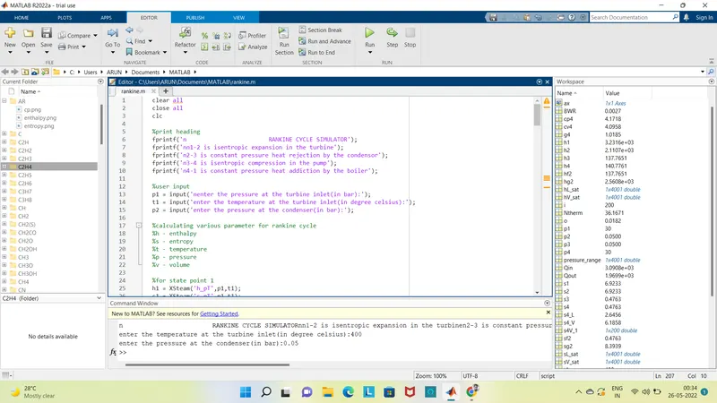
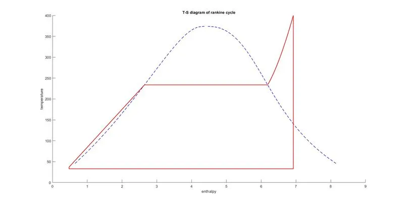
OUTPUTS :
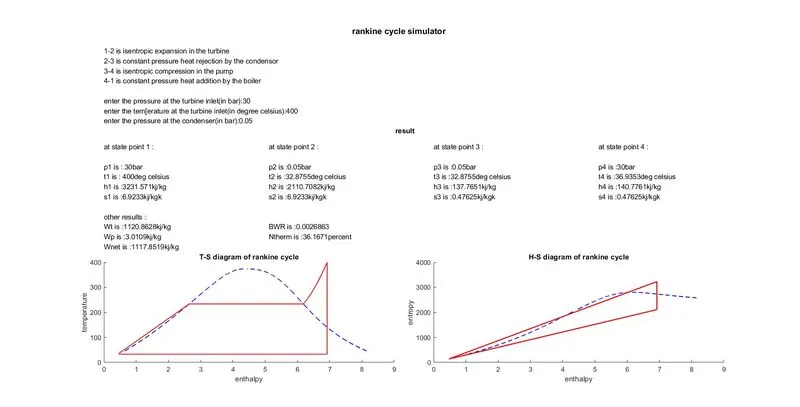
Results :
Reference :
1.https://skill-lync.com/student-projects/matlab-project-rankine-cycle-simulator
2.https://energyeducation.ca/encyclopedia/Rankine_cycle
3.https://youtu.be/QFZN71MY71o
4.https://www.thermal-engineering.org/what-is-rankine-cycle-steam-turbine-cycle-definition/