Project 2 - Rankine cycle Simulator

clc
clear all
close all
% giving description to all process

fprintf("Rankine cycle simulator \n");

 %input from user

P1 = input ("\n Enter the turbine inlet pressure (in bar): ");
T1 = input ("\n Enter the turbine inlet temperature (Degree celcius): ");
P2 = input ("\n Enter the turbine  pressure (in bar): ");
fprintf("\n")

%disp(P1)
%disp(T1)
%disp(P2)

% results
 %calculating requires values at all states point

% At state point 1


%entrophy
S1 = XSteam("s_pT",P1,T1);
##fprintf("S1 is : %f kJ/kg \n", S1)

% enthalpy
H1 = XSteam("h_pT",P1,T1);
##fprintf("H1 is : %f kJ/kg \n", H1)

% At state point 2


S2=S1;
##fprintf("S1 is : %f kJ/kg \n", S2)

% saturated liquid entropy
sf2=XSteam('sL_p',P2);

% saturated vapour entropy
sg2=XSteam('sV_p',P2);

% staturated liquid enthalpy
hf2=XSteam('hL_p',P2);

% saturated vapour enthalpy
hg2=XSteam('hV_p',P2);

% temperature at state 2
T2=XSteam('Tsat_p',P2)
x2=((S2-sf2)/(sg2-sf2))

% enthalpy at state 2
H2=hf2+(x2*(hg2-hf2))


% At state point 3


P3=P2
T3 = XSteam('Tsat_p',P3);
S3 = XSteam('sL_p',P3);
H3 =XSteam('hL_p',P3)

%to calculate  gama (k)

% specific heat at constant pressure
Cp = XSteam('cpL_p',P3)

% specific heat at constat volume
Cv = XSteam('cvL_p', P3)

k = (Cp/Cv)


% at state point 4


P4=P1
S4=S3

% enthaloy as afunction of of pressure and temperature
H4 = XSteam('h_ps',P4,S4);

T4=T3*((P4/P3)^((k-1)/k))

%work done by turbine

Wt=H1-H2;

% work done to run pump

Wp=H4-H3;

%net work done

Wnet=Wt-Wp

% heat into system

Qin = H1 -H4

% heat out system

Qout = H2-H3

% thermal efficiency

Eff = (Wnet/Qin)

% specific steam consumption

%  SSC = mass flow rate/power

SSC=3600/Wnet

% BACK WORK RATIO

back_work_ratio = Qin/Qout;


% At state point 5 and 6

T5 = XSteam('Tsat_p',P1);
T6=T5;
S5 = XSteam('sL_p',P1);
S6 = XSteam('sV_p',P1);
H5 = XSteam('hL_p',P1)
H6 = XSteam('hL_p',P1)


%fprintf('H1 is : %f kJ/kg n', H1)

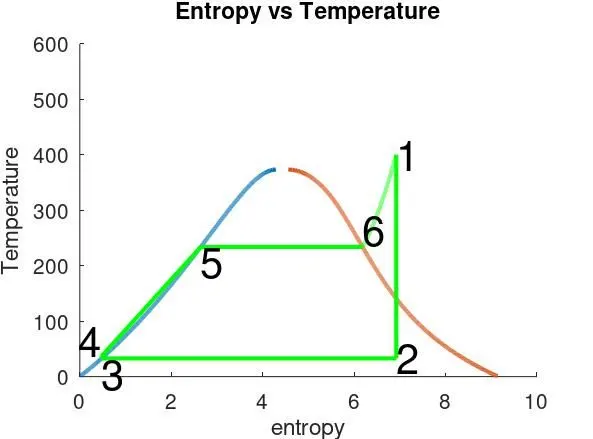
% temperature vs entropy  graph

% plot saturation liquid and vapour line
figure(1)
Temperature_1 = linspace(0,T1,500);
for j = 1:length(Temperature_1)
      H_L(j) = XSteam('hL_T',Temperature_1(j));
      H_V(j) = XSteam('hV_T',Temperature_1(j));
      S_L(j) = XSteam('sL_T',Temperature_1(j));
      S_V(j) = XSteam('sV_T',Temperature_1(j));
end

hold on

% plotting saturated liquid entropy vs temperature
plot (S_L,Temperature_1,'linewidth',2)

% plotting saturated vapour entropy vs temperature
plot (S_V,Temperature_1,'linewidth',2)
xlabel ('entropy')
ylabel ('Temperature')
title ('Entropy vs Temperature')

Temperature_2 = linspace(T6,T1,500);
    for   f=1:length(Temperature_2)
          S(f)=XSteam('s_pT',P1,Temperature_2(f));

    end
  hold on

% plotting entropy vs enthalpy
  plot ([S1 S2 S3 S4 S5 S6 S],[T1 T2 T3 T4 T5 T6 Temperature_2],'linewidth',2,'color','g')
  axis ([0 10 0 600])
  text (S1,T1,'1','Fontsize',20)
  text (S2,T2,'2','Fontsize',20)
  text (S3,T3,'3','Fontsize',20,'verticalalignment','top')
  text (S4,T4,'4','Fontsize',20,'verticalalignment','bottom','horizontalalignment','right')
  text (S5,T5,'5','Fontsize',20,'verticalalignment','top')
  text (S6,T6,'6','Fontsize',20,'verticalalignment','bottom','horizontalalignment','left')


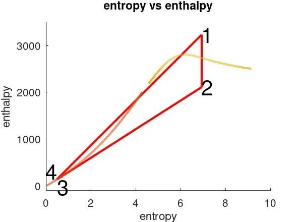
% entropy vs enthalpy  graph

figure (2)

hold on

% plotting entropy vs enthalpy
plot([S1 S2 S3 S4 S1],[H1 H2 H3 H4 H1],'linewidth',2,'color','r')
axis ([0 10 -100 3500])
  text (S1,H1,'1','Fontsize',20)
  text (S2,H2,'2','Fontsize',20)
  text (S3,H3,'3','Fontsize',20,'verticalalignment','top')
  text (S4,H4,'4','Fontsize',20,'verticalalignment','bottom','horizontalalignment','right')

% plotting entropy vs enthalpy at liquid phase
plot(S_L,H_L,'linewidth',2)

% plotting entropy vs enthalpy at liquid phase
plot(S_V,H_V,'linewidth',2)
xlabel('entropy')
ylabel ('enthalpy')
title ('entropy vs enthalpy')

% results

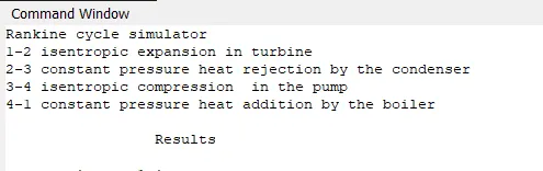
fprintf("Rankine cycle simulator \n");
fprintf("1-2 isentropic expansion in turbine \n");
fprintf("2-3 constant pressure heat rejection by the condenser \n");
fprintf("3-4 isentropic compression  in the pump \n");
fprintf("4-1 constant pressure heat addition by the boiler \n");

fprintf("\n")

fprintf ("\t\t Results \t \n")

fprintf("\n")

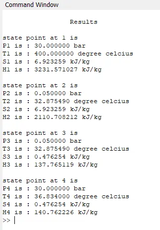
fprintf("state point at 1 is \n");
fprintf("P1 is : %f bar \n",P1);
fprintf("T1 is : %f degree celcius \n",T1);
fprintf("S1 is : %f kJ/kg \n", S1)
fprintf("H1 is : %f kJ/kg \n", H1)

fprintf("\n")

fprintf("state point at 2 is \n");
fprintf("P2 is : %f bar \n",P2);
fprintf("T2 is : %f degree celcius \n",T2);
fprintf("S2 is : %f kJ/kg \n", S2)
fprintf("H2 is : %f kJ/kg \n", H2)

fprintf("\n")

fprintf("state point at 3 is \n");
fprintf("P3 is : %f bar \n",P3);
fprintf("T3 is : %f degree celcius \n",T3);
fprintf("S3 is : %f kJ/kg \n", S3)
fprintf("H3 is : %f kJ/kg \n", H3)

fprintf("\n")

fprintf("state point at 4 is \n");
fprintf("P4 is : %f bar \n",P4);
fprintf("T4 is : %f degree celcius \n",T4);
fprintf("S4 is : %f kJ/kg \n", S4)
fprintf("H4 is : %f kJ/kg \n", H4)