Project 2 - Rankine cycle Simulator

Aim:

• To create a Rankine Cycle Simulator using OCTAVE/MATLAB.
• The code should calculate the state points of the Rankine Cycle (any type of your choice) based on user inputs. 
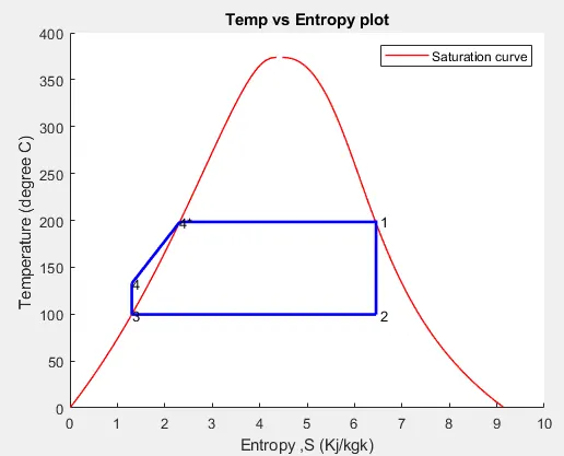
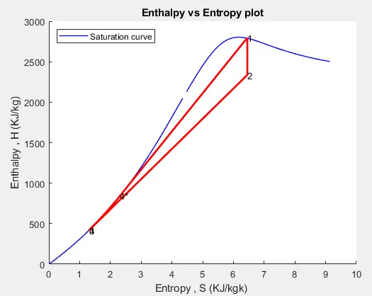
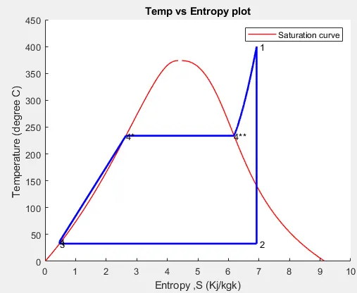
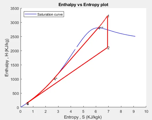
• Later, plot the corresponding T-s and h-s plots for the given set of inputs. Title and axes labels are a must, while legends could be used if necessary.

Theory:

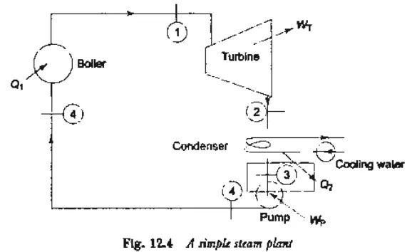
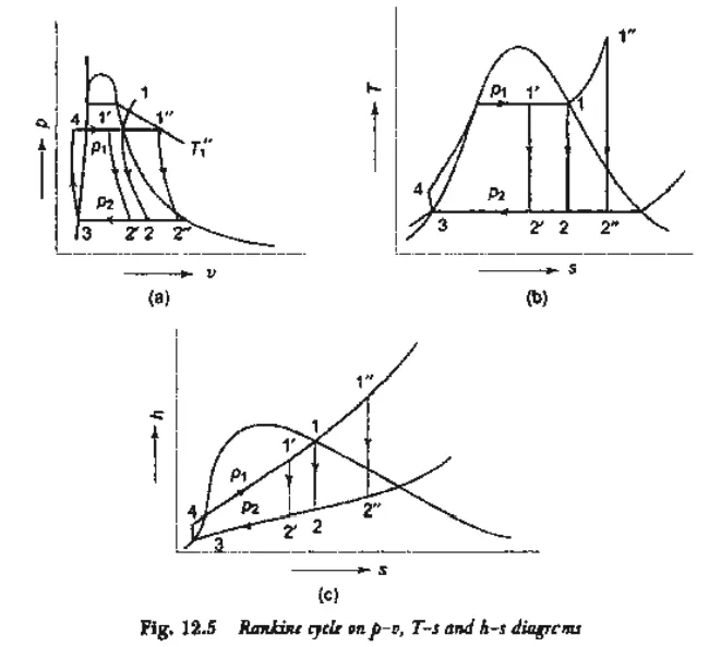
For each process in the vapour power cycle., it is possible to assume a hypothetical or ideal process which represents the basic intended operation and involves no extraneous effects. For the steam boiler, this would be a reversible constant pressure heating process of water to form steam, for the turbine the ideal process would be a revenible adiabatic expansion of steam, for the condenser it would be a reversible constant pressure heat rejection as the steam condenses till it becomes saturated liquid, and for the pump, the ideal process would be the reversible adiabatic compression of this liquid ending at the initial pressure. When all these four processes are ideal, the cycle is an ideal cycle, called a Rankine cycle. This is a reversible cycle. Figure 12.4 shows the flow diagram of the Rakine cycle, and in .Fig. 12.5, the cycle has been plotted on the p-v, T-s, and h-s planes. The numbers on the plots correspond to the numbers on the flow diagram. For any given pressure, the steam approaching the turbine may be dry saturated (state l) wet (state l '), or superheated (state l"), but the fluid approaching lhe pump is, in each case, saturated liquid {state 3). Steam expands reversibly and adiabiatically in the turbine from state 1 to state 2 (or I' to 2', or l" to 2"), the steam leaving the turbine condenses to water in tbe condenser reversibly at constant pressure from state 2 (or 2', or 2") to state 3, the water at state 3 is then pumped to the boiler at state 4 reversibly and adiabatically, and the water is heated in the boiler to from steam reversibly at constant pressure from state 4 to state I (or I' or I").

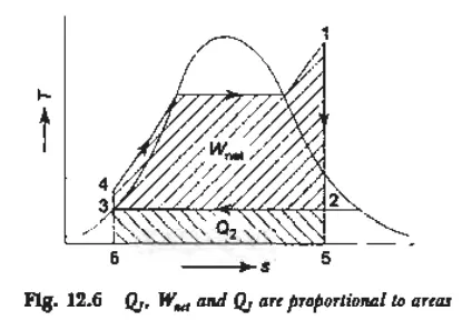
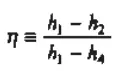
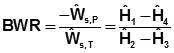
The ratio of the compressor work to the turbine work is called the back-work ratio. Sometimes, more than one-half of the turbine work may be used by the compressor.

https://www.learnthermo.com/T1-tutorial/ch09/lesson-B/pg07.php

Steam table:

https://drive.google.com/file/d/1RK_fvrOj38CIaQvmLT1S3daqHnxKCGU-/view

Code:

Explaination:

1. This is a matlab code, the first few lines of code is used to display a bunch of statements and the second part of the same block of code is used to take user inputs which will later be used for further calculations.
2. The code also talks about the various stages of the Rankine cycle, it is important to note that the values imported into the main code from the function code should be done with atmost care.
3. The appropriate values of enthalpy and entropy are called and then the the dryness fraction of the steam is calculated, further the enthalpy values are calculated at state 2.
4. The work done by the turbine is calculated along with the work done by the pump. Later the net work done is calculated along with Qin and Qout.
5. Back Work ratio, Specific steam consumption, thermal effeciency are also calculated.
6. The next set of code has the function of generating state points like: Temperature, entropy and enthalpy.
7. The next set of code is used to generate the saturation curve for the T-s diagram and H-s diagram.
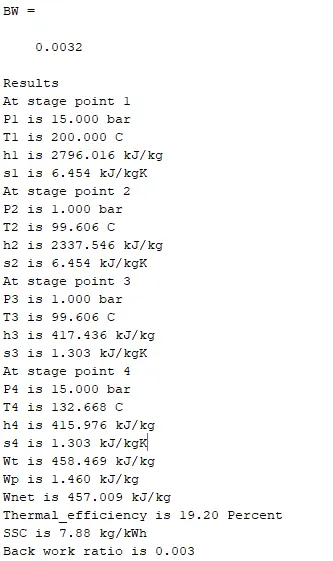
8. The final step is to print all the values in the command window.

clear all
close all
clc

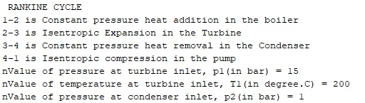
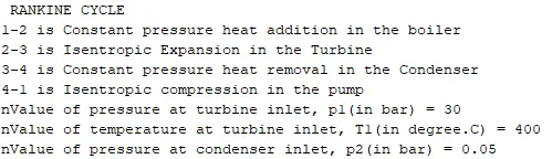
disp(' RANKINE CYCLE ');
disp('1-2 is Constant pressure heat addition in the boiler');
disp('2-3 is Isentropic Expansion in the Turbine');
disp('3-4 is Constant pressure heat removal in the Condenser');
disp('4-1 is Isentropic compression in the pump');
p1 = input('nValue of pressure at turbine inlet, p1(in bar) = ');
T1 = input('nValue of temperature at turbine inlet, T1(in degree.C) = ');
p2 = input('nValue of pressure at condenser inlet, p2(in bar) = ');

% At State 1
h1 = XSteam('h_pT', p1, T1); % Extracting Enthalpy at state pt 1
s1 = XSteam('s_pT', p1, T1); % Similarly

% At State 2
s2 = s1; % Isentropic Expansion
sf2= XSteam('sL_p', p2); % Saturated Liquid Entropy
sg2 = XSteam('sV_p', p2); % Saturated Vapour Entropy
x2 = (s2-sf2)/(sg2-sf2); 
hf2 = XSteam('hL_p', p2); % Saturated liquid enthalpy
hg2 = XSteam('hV_p', p2); % Saturated vapour enthalpy
h2 = hf2 + (x2*(hg2-hf2));

% At State 3
p3 = p2; % Constant pressure Heat rejection in Condenser
s3= XSteam('sL_p', p3); % Saturated Liquid Entropy
h3 = XSteam('hL_p', p3); % Saturated liquid enthalpy

% At State 4
s4 = s3; % isentropic compression process
p4 = p1; % constant pressure heat rejection

% Work done by turbine
Wt = h1 - h2;
% Work done to run pump
v3 = XSteam('vL_p', p3); % saturated liquid vapour at pressure 3
Wp = v3*(p4 - p3)*100; % work done for pump
h4 = h3 - Wp;
%Net work
Wnet = Wt - Wp;
%Heat into the system
Qin = h1 - h4;
%Heat out of the system
Qout = h2 - h3;
%Thermal efficiency
thermal_eff = (Wnet/Qin)*100;
%Specific Steam Consumption
%SSC = mass flow rate/power
SSC = (3600/Wnet);
% Back Work ratio
BW = (Wp/Wt)

% Calculation of Temperatures at the state points
T3 = XSteam('Tsat_p', p3);
T2 = T3;
Cp4 = XSteam('Cp_ps', p4, s4);
Cv4 = XSteam('Cv_ps', p4, s4);
k = Cp4/Cv4;
T4 = T3/((p3/p4)^((k-1)/k));
%Calculating Temperature, Entropy and Enthalpy at the vapour and liquid line for plotting
T6 = XSteam('Tsat_p', p1);
s5 = XSteam('sL_p', p1);
s6 = XSteam('sV_p', p1);
h5 = XSteam('hL_p', p1);
h6 = XSteam('hV_p', p1);
%
if (T6==0)
    printf('The cycle can not have %f as inlet temperature', T6);
end
T5 = T6;

%Plotting the saturation curve
T = linspace(1,375,1000);
for i = 1:length(T)
sf(i) = XSteam('sL_T', T(i));
sg(i) = XSteam('sV_T', T(i));
hf(i) = XSteam('hL_T', T(i));
hg(i) = XSteam('hV_T', T(i));
end
%Plotting T-s diagram
figure(1)
hold on
plot(sf, T, 'r','linewidth',1)
plot(sg, T, 'r','linewidth',1)
plot([s1 s2], [T1 T2], 'b', 'linewidth', 2)
plot([s2 s3], [T2 T3] ,'b', 'linewidth', 2)
plot([s3 s4], [T3 T4], 'b', 'linewidth', 2)
plot([s4 s5], [T4 T5], 'b', 'linewidth', 2)
plot([s5 s6], [T5 T6], 'b', 'linewidth', 2)
sc1 = linspace(s6, s1, 1000);

for l = 1:length(sc1)
 Tc1(l) = XSteam('T_ps', p1, sc1(l));
end
plot(sc1, Tc1, 'b', 'linewidth', 2)
text(s1+0.1, T1, '1')
text(s2+0.1, T2, '2')
text(s3, T3, '3')
text(s4, T4, '4')
text(s5, T5, '4*')
text(s6, T6, '4**')
title('Temp vs Entropy plot')
xlabel('Entropy ,S (Kj/kgk)')
ylabel('Temperature (degree C) ')
legend('Saturation curve')
%Plotting h-s diagram
figure(2)
hold on
plot(sf, hf, 'b', 'linewidth', 1)
plot(sg, hg, 'b', 'linewidth', 1)
plot([s1 s2], [h1 h2], 'r', 'linewidth', 2)
plot([s2 s3], [h2 h3], 'r', 'linewidth', 2)
plot([s3 s4], [h3 h4], 'r', 'linewidth', 2)
hc = linspace(h4, h5, 100);

for r = 1:length(hc)
sch(r) = XSteam('s_ph', p1, hc(r));
end
plot(sch,hc, 'r', 'linewidth', 2)
plot([s5 s6], [h5 h6], 'r', 'linewidth', 2)
for m = 1:length(sc1)
hc1(m) = XSteam('h_ps', p1, sc1(m));
end
plot(sc1, hc1, 'r', 'linewidth', 2)
text(s1, h1, '1')
text(s2, h2, '2')
text(s3, h3, '3')
text(s4, h4, '4')
text(s5, h5, '4*')
text(s6, h6, '4**')
title('Enthalpy vs Entropy plot')
xlabel('Entropy , S (KJ/kgk) ')
ylabel('Enthalpy , H (KJ/kg)')
legend('Saturation curve','location','northwest')

% Displaying the Results in the Command Window:
disp('Results');
p1 = p1;
T1 = T1;
p2 = p2;
disp('At stage point 1');
n1 = sprintf('P1 is %.3f bar',p1);
disp(n1);
n2 = sprintf('T1 is %.3f C',T1);
disp(n2);
n3 = sprintf('h1 is %.3f kJ/kg',h1);
disp(n3);
n4 = sprintf('s1 is %.3f kJ/kgK',s1);
disp(n4);
disp('At stage point 2');
n11 = sprintf('P2 is %.3f bar',p2);
disp(n11);
n21 = sprintf('T2 is %.3f C',T2);
disp(n21);
n31 = sprintf('h2 is %.3f kJ/kg',h2);
disp(n31);
n41 = sprintf('s2 is %.3f kJ/kgK',s2);
disp(n41);
disp('At stage point 3');
n12 = sprintf('P3 is %.3f bar',p3);
disp(n12);
n22 = sprintf('T3 is %.3f C',T3);
disp(n22);
n32 = sprintf('h3 is %.3f kJ/kg',h3);
disp(n32);
n42 = sprintf('s3 is %.3f kJ/kgK',s3);
disp(n42);
disp('At stage point 4');
n13 = sprintf('P4 is %.3f bar',p4);
disp(n13);
n23 = sprintf('T4 is %.3f C',T4);
disp(n23);
n33 = sprintf('h4 is %.3f kJ/kg',h4);
disp(n33);
n43 = sprintf('s4 is %.3f kJ/kgK',s4);
disp(n43);
n14 = sprintf('Wt is %.3f kJ/kg',Wt);
disp(n14);
n15 = sprintf('Wp is %.3f kJ/kg',Wp);
disp(n15);
n16 = sprintf('Wnet is %.3f kJ/kg',Wnet);
disp(n16);
n17 = sprintf('Thermal_efficiency is %.2f Percent',thermal_eff);
disp(n17);
n18 = sprintf('SSC is %.2f kg/kWh',SSC);
disp(n18);
n19 = sprintf('Back work ratio is %.3f ',BW);
disp(n19);

Plots:

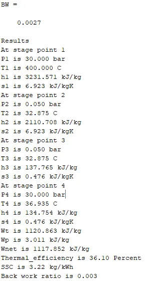
Inputs:
Turbine Inlet temperature = 400° C
Turbine Inlet Pressure = 30 bars
Turbine Outlet Pressure = 0.05 bars = Condenser Inlet Pressure

Inputs:
Turbine Inlet temperature = 200° C
Turbine Inlet Pressure = 15 bars
Turbine Outlet Pressure = 1 bars = Condenser Inlet Pressure