Project 2 - Rankine cycle Simulator

Objective :

To create a Matlab program to solve the Rankine cycle and to obtain the state values for the cycle with the help of XSteam Library. Also, to plot T-S & H-S graph for the values generated in the program.

Introduction :

The Rankine cycle is an idealized thermodynamic cycle describing the process by which certain heat engines, such as steam turbines or reciprocating steam engines, allow mechanical work to be extracted from a fluid as it moves between a heat source and heat sink.

The processes taking place in a Rankine cycle are as follows;

• Process 1–2: The working fluid is pumped from low to high pressure. As the fluid is a liquid at this stage, the pump requires little input energy. Process 1-2 is isentropic compression.
• Process 2–3: The high-pressure liquid enters a boiler, where it is heated at constant pressure by an external heat source to become a dry saturated vapour. The input energy required can be easily calculated graphically, using an enthalpy-entropy chart (h-s chart or Mollier diagram), or numerically, using steam tables or software. Process 2-3 is constant pressure heat addition in boiler.
• Process 3–4: The dry saturated vapour expands through a turbine, generating power. This decreases the temperature and pressure of the vapour, and some condensation may occur. The output in this process can be easily calculated using the chart or tables noted above. Process 3-4 is isentropic expansion.
• Process 4–1: The wet vapour then enters a condenser, where it is condensed at a constant pressure to become a saturated liquid. Process 4-1 is constant pressure heat rejection in condenser.

Formulas :

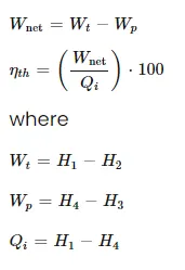
• Net Work Done & Efficiency;

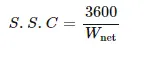
• Specific Steam Consumption;

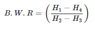
• Back Work Ratio;

The program to solve the Rankine cycle is mentioned below;

clear all%1%
close all
clc

fprintf('%75s\n\n','RANKINE CYCLE SIMULATOR');%2%
fprintf('1-2 is Isentropic expansion in Turbine\n');
fprintf('2-3 is Isobaric heat rejected by Condenser\n');
fprintf('3-4 is Isentropic compression in PUMP\n');
fprintf('4-1 is isobaric heat addition by the Boiler\n\n');

P1=input('Enter the Pressure at the Turbine Inlet(in bar):');%3%
T1=input('Enter the Temperature at the Turbine Inlet(in degree):');
P2=input('Enter the Pressure at Condenser(in bar):');

S1=XSteam('s_pT',P1,T1);%4%
H1=XSteam('h_pT',P1,T1);

S2=S1;%5%
sf2=XSteam('sL_p',P2);
sg2=XSteam('sV_p',P2);
hf2=XSteam('hL_p',P2);
hg2=XSteam('hV_p',P2);

T2=XSteam('Tsat_p',P2);
x2=((S2-sf2)/(sg2-sf2));

H2=hf2+(x2*(hg2-hf2));

P3=P2;%6%
T3=XSteam('Tsat_p',P3);
S3=XSteam('sL_p',P3);
H3=XSteam('hL_p',P3);

cp=XSteam('cpL_p',P3);%7%
cv=XSteam('cvL_p',P3);
gamma=(cp/cv);

P4=P1;%8%
S4=S3;
H4=XSteam('h_ps',P4,S4);
T4=T3*((P4/P3)^((gamma-1)/gamma));

Wt=H1-H2;%9%
Wp=H4-H3;
W_net=Wt-Wp;

q_in=H1-H4;%10%
q_out=H2-H3;

n=W_net/q_in;%11%
n_percent=n*100;

SSC=3600/W_net;%12%

BWR=q_in/q_out;%13%

T5=XSteam('Tsat_p',P1);%14%
T6=T5;
S5=XSteam('sL_p',P1);
S6=XSteam('sV_p',P1);
H5=XSteam('hL_p',P1);
H6=XSteam('hV_p',P1);

figure(1)%15%
T_Zone1=linspace(T5,T1,500);

for i=1:length(T_Zone1)
    S(i)=XSteam('s_pT',P1,T_Zone1(i));
end
hold on
plot([S1 S2 S3 S4 S5 S6 S],[T1 T2 T3 T4 T5 T6 T_Zone1],'linewidth',3,'color','k')
axis([0 10 0 430])
text(S1,T1,'1','FontSize',15)
text(S2,T2,'2','FontSize',15)
text(S3,T3,'3','FontSize',15,'VerticalAlignment','top')
text(S4,T4,'4','FontSize',15,'VerticalAlignment','bottom','HorizontalAlignment','right')
text(S5,T5,'5','FontSize',15,'VerticalAlignment','top')
text(S6,T6,'6','FontSize',15,'VerticalAlignment','top','HorizontalAlignment','right')

T_Zone2=linspace(0,T1,500);
for j=1:length(T_Zone2)
    sl(j)=XSteam('sL_T',T_Zone2(j));
    sv(j)=XSteam('sV_T',T_Zone2(j));
    hl(j)=XSteam('hL_T',T_Zone2(j));
    hv(j)=XSteam('hV_T',T_Zone2(j));
end
plot(sl,T_Zone2,'linewidth',1.5,'color','r')
plot(sv,T_Zone2,'linewidth',1.5,'color','r')
xlabel('Entropy')
ylabel('Temperature')
title('Entropy vs Temperature')
hold off

figure(2)%16%
hold on
plot([S1 S2 S3 S4 S1],[H1 H2 H3 H4 H1],'linewidth',3,'color','k')
axis([0 10 -100 3500])
text(S1,H1,'1','FontSize',15)
text(S2,H2,'2','FontSize',15)
text(S3,H3,'3','FontSize',15,'VerticalAlignment','top','HorizontalAlignment','left')
text(S4,H4,'4','FontSize',15,'VerticalAlignment','bottom','HorizontalAlignment','right')

plot(sv,hv,'linewidth',1.5,'color','r')
plot(sl,hl,'linewidth',1.5,'color','r')
xlabel('Entropy')
ylabel('Enthalpy')
title('Entropy vs Enthalpy')

fprintf('\n At State Point 1 :\n');%17%
fprintf('P1 is : %f Bar\n',P1);
fprintf('T1 is : %f Deg Celcius\n',T1);
fprintf('H1 is : %f KJ/kg\n',H1);
fprintf('S1 is : %f KJ/kgK\n',S1);

fprintf('\n At State Point 2 :\n');
fprintf('P2 is : %f Bar\n',P2);
fprintf('T2 is : %f Deg Celcius\n',T2);
fprintf('H2 is : %f KJ/kg\n',H2);
fprintf('S2 is : %f KJ/kgK\n',S2);
fprintf('X2 is : %f\n',x2);

fprintf('\n At State Point 3 :\n');
fprintf('P3 is : %f Bar\n',P3);
fprintf('T3 is : %f Deg Celcius\n',T3);
fprintf('H3 is : %f KJ/kg\n',H3);
fprintf('S3 is : %f KJ/kgK\n',S3);

fprintf('\n At State Point 4 :\n');
fprintf('P4 is : %f Bar\n',P4);
fprintf('T4 is : %f Deg Celcius\n',T4);
fprintf('H4 is : %f KJ/kg\n',H4);
fprintf('S4 is : %f KJ/kgK\n',S4);

fprintf('Wt : %f KJ/kg\n',Wt);
fprintf('Wp : %f KJ/kg\n',Wp);
fprintf('Wnet : %f KJ/kg\n',W_net);
fprintf('Ntherm : %f percent\n',n_percent);
fprintf('SSC : %f kg/KWh',SSC);
fprintf('BWR : %f\n',BWR);

Stepwise Explanation :

1-The first 3 lines are used to clear & close all the previous data, to avoid mixing of previous data with the latest data.

2-The next few lines are used to print the process of rankine cycle.

3-The next few lines are used to obtain the input values to calculate the other necessary values.

4-These lines are used to obtain the state 1 values for entropy & enthalpy.

5-These lines are used to obtain the state 2 values.

6-These lines are used to obtain the state 3 values.

7-These lines are used to obtain the gamma value, to calculate the state 4.

8-These lines are used to obtain the state 4 values.

9-These lines are used to find out the net work done in the process.

10-These lines are used to find out the heat addition & rejection values.

11-These lines help us to find the efficiency of the cycle.

12-This line is used to calculate the Specific Steam Consumption.

13-This line is used to calculate the Back Work Ratio.

14-These lines are used to obtain the entropy & enthalpy values for superheated steam condition.

15-The following lines are used to generate a T-S graph for the given input values.

16-The following lines are used to generate a H-S graph for the given input values.

17-The following lines are used to print the output values of each state,net work done,efficiency,SSC & BWR.

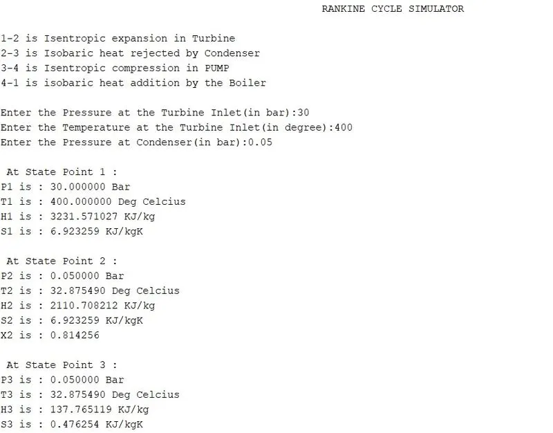
Output :

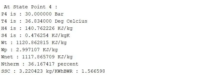
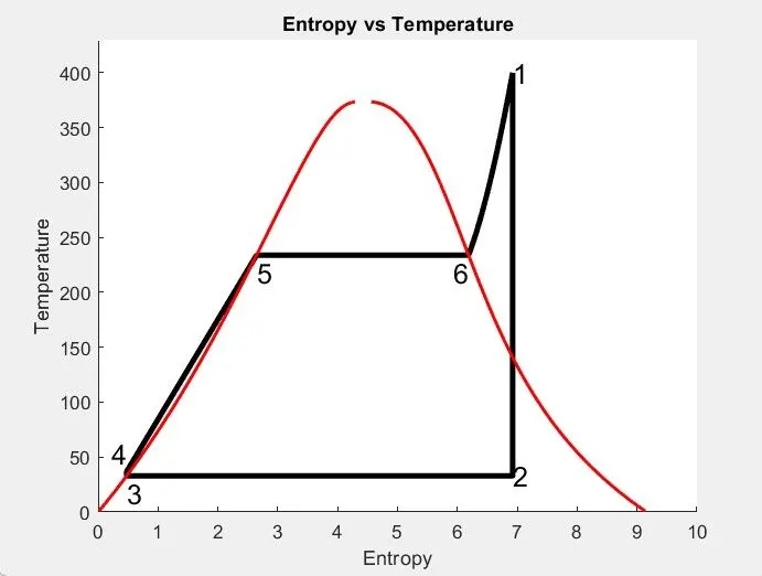
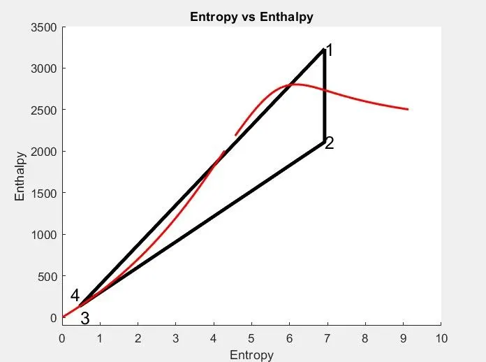
Errors faced during programming :

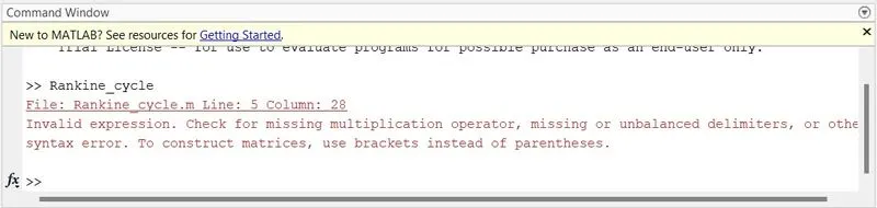
The above error indicates that instead of declaring the heading as a string value, i had declared it as an object.

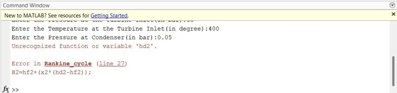
The above error indicates that a variable is wrongly declared & no value is assigned to it. Therefore, the variable had to be changed from hd2 to hg2.