Project 2 - Rankine cycle Simulator
A Rankine Cycle Simulator using MATLAB
clear all
close all
clear all
clc

fprintf(' RANKINE CYCLE STIMULATOR\n')

fprintf('1-2 Isentropic Expansion in the Turbine\n')
fprintf('2-3 Constant Pressure Heat Rejection by the Condenser\n')
fprintf('3-2 Isentropic Compression in the Pump\n')
fprintf('4-1 Constant Pressure Heat Addition by the Boiler\n')
%inputs

P1 = input('Enter the Pressure at the Turbine Inlet (in bar): ');
T1 = input('Enter the Temperature at the Turbine inlet (in Degree celsius): ');
P2 = input('Enter the Pressure at the Condenser (in bar): ');

disp( 'RESULTS')
%for vapour

high_cpV= XSteam('CpV_p', P1);

low_cpV=XSteam('CpV_p', P2);

high_cvV=XSteam('CvV_p', P1);

low_cvV=XSteam('CvV_p', P2);
% for liquid
high_cpL= XSteam('CpL_p', P1);

low_cpL=XSteam('CpL_p', P2);

high_cvL=XSteam('CvL_p', P1);

low_cvL=XSteam('CvL_p', P2);


%for high pressure

T1s = XSteam('Tsat_p', P1);
S1g = XSteam('sV_p', P1);
S1f = XSteam('SL_p', P1);
S1fg = S1g - S1f;

H1f = XSteam('hL_p', P1);
H1g = XSteam('hV_p', P1);
H1fg = H1g - H1f;

%for low pressure

S2g = XSteam('sV_p', P2);
S2f = XSteam('SL_p', P2);
S2fg = S2g - S2f;

T2s = XSteam('Tsat_p', P2);
H2f = XSteam('hL_p', P2);
H2g = XSteam('hV_p', P2);
H2fg = H2g - H2f;

%% state point 1

disp('At state point 1:')

fprintf('P1 is : %f Bar\n', P1)

fprintf('T1 is : %f Deg celsius\n', T1)

H1 = XSteam('h_pt', P1, T1);
fprintf('H1 is : %f kJ/kg\n', H1)

S1 = XSteam('s_pt', P1, T1);
fprintf('S1 is : %f kJ/kgK\n', S1)
%% state point 2

disp('At state point 2:')

fprintf('P2 is : %f Bar\n', P2)
S2 = S1;
fprintf('S2 is : %f kJ/kgK\n', S2)
%predicting location of point 2 in T-s
if (S2<=S2g)
    X2 = (S2 - S2f) / (S2fg);
else
X2=1;
end
fprintf('x2 is :%f \n', X2)
if(X2<1)
T2=T2s;
else
%t2 cal by s2=s2g+low_cpV*(log(T2/T2s))
T2=(T2s+273.15)*exp((S2-S2g)/low_cpV) ;
T2=T2-273.15;
end
fprintf('T2 is : %f Deg celsius \n', T2)

if (X2<1)
H2 = H2f + X2 * H2fg;

else
H2=H2g+ low_cpV*(T2-T2s);

end

fprintf('H2 is : %f kJ/kg\n', H2)

%% state point 3
% no subcooling in condensor

disp('At state point 3:')

P3= P2;
fprintf('P3 is : %f Bar\n', P3)

V3 = XSteam('vL_p', P3);
T3= T2s;
fprintf('T3 is : %f Deg celsius\n', T3)

H3 =H2f;
fprintf('H3 is : %f kJ/kg\n', H3)

S3 =S2f;
fprintf('S3 is : %f kJ/kgK\n', S3)

%% state point 4
disp('at state point 4:')

P4 = P1;
fprintf('p4 is : %f Bar\n', P4)

S4 = S3;
fprintf('s4 is : %f kJ/kgK\n', S4)

Wp = V3 * (P4 - P3) * 100;
H4 = Wp + H3;
fprintf('H4 is : %f kJ/kg\n', H4)
% to cal T4 s4=s3=sf1-high_cpL*1n(tis/t4)

term=exp((S1f-S4)/high_cpL);
T4= T1s/term;

fprintf('T4 is : %f Deg celsius \n', T4)
%% work done, heat, SSC and efficiency calculations
Wt = H1 - H2;

fprintf('Work by turbine is : %f kJ/kg\n', Wt)
fprintf('Work by compressor is : %f kJ/kg\n', Wp)
Wnet = Wt - Wp;

fprintf('Net Wok done is : %f kJ/kg\n', Wnet)

Qin = H1 - H4;

eff_thermal = (Wnet / Qin)*100;
fprintf('Thermal efficiency is : %f', eff_thermal); disp('%')
SSC = 3600 / Wt;
fprintf('S.S.c is : %f kg/kwh ', SSC)

% Calculation for plotting Liquid and vapour lines
% <>

temp = linspace(1, 373, 500);

for i = 1: length(temp)
H_L(i) = XSteam('hL_T', temp(i));
H_V(i) = XSteam('hV_T', temp(i));
S_L(i) = XSteam('sL_T', temp(i));
S_V(i) = XSteam('sv_T', temp(i));

end
%% Ploting T - S and H - S Diagrams

figure(1)
hold on

plot([S1 S2], [T1 T2], 'k', 'linewidth', 1.5)
text(S1,T1,'1')

text(S2,T2,'2' )

plot([S2 S2g], [T2 T2s], 'k', 'linewidth', 1.5)

text(S2g,T2s,' 2s')

plot([S2g S3], [T2s T3], 'k', 'linewidth', 1.5)

text(S3,T3,'3')

plot([S3 S4], [T3 T4], 'k', 'linewidth', 1.5)

text (S4,T4,'4')

plot([S4 S1f], [T4 T1s], 'k','linewidth', 1.5)

text(S1f,T1s,'4s')

plot([S1f S1g], [T1s T1s], 'k', 'linewidth', 1.5)

text(S1g,T1s,'1s')

plot([S1g S1], [T1s T1], 'k', 'linewidth', 1.5)

plot(S_L, temp, 'r','linewidth', 2.5)

plot(S_V, temp, 'r', 'linewidth', 2.5)

% direction

text(S1,(T1+T2)/2, 'vee', 'HorizontalAlignment', 'center', 'color','m')
text((S2g+S2f)/2,T3, 'langle', 'color','m')

text(S3, (T3+T4)/2, 'wedge', 'Horizontalalignment', 'center', 'color', 'm')
text((S1f+S1g)/2,T1s, 'rangle', 'color','m')

title('T-S Diagram of Ideal Rankine Cylce')

ylabel('Temprature (degc)')

xlabel('Specific Entropy (kJ/kgk)')
figure(2) % H-S
hold on

plot([S1 S2], [H1 H2], 'k', 'linewidth', 1);
text(S1,H1,'1')

plot([S2 S3], [H2 H3], 'k', 'linewidth', 1);
text(S2,H2,'2')

plot([S3 S4], [H3 H4], 'k', 'linewidth', 1);
text(S3,H3,'3')

plot([S4 S1], [H4 H1], 'k', 'linewidth', 1);
text(S4,H4,'4')

plot(S_L, H_L, 'r', 'linewidth', 3)
plot(S_V, H_V, 'r','linewidth',3)
title('H-S Diagram', 'FontSize', 15)

ylabel('Specific enthalpy (kJ/kg)')

xlabel('Specific Entropy (kJ/kgk)')
strt the pgm with outputs or the inputs from the user, use the data given. state the points1,2,3,4 amd the work done and ssc nd efficiency calculations ,plot t-s and h-s, plot the diagrams
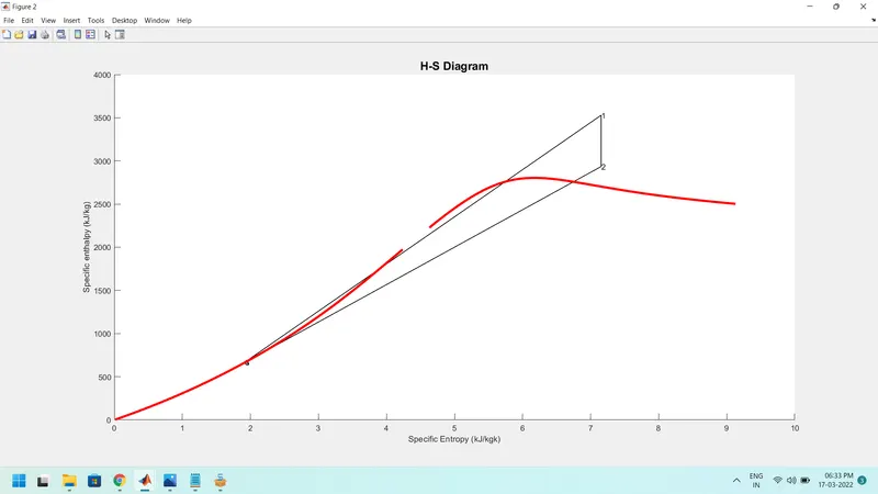
H-S Diagram
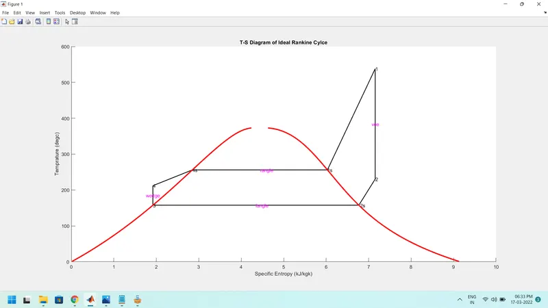
T-S diagram
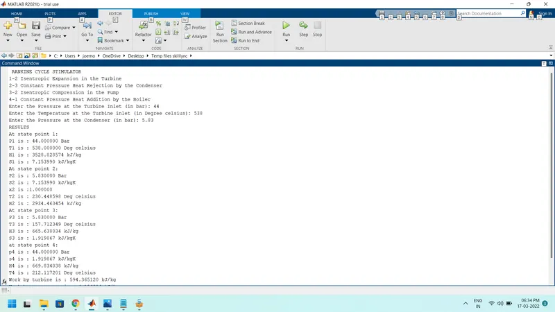
Command window
RANKINE CYCLE STIMULATOR
1-2 Isentropic Expansion in the Turbine
2-3 Constant Pressure Heat Rejection by the Condenser
3-2 Isentropic Compression in the Pump
4-1 Constant Pressure Heat Addition by the Boiler
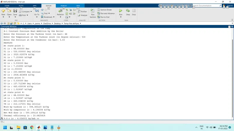
Enter the Pressure at the Turbine Inlet (in bar): 44
Enter the Temperature at the Turbine inlet (in Degree celsius): 538
Enter the Pressure at the Condenser (in bar): 5.83
RESULTS
At state point 1:
P1 is : 44.000000 Bar
T1 is : 538.000000 Deg celsius
H1 is : 3528.828574 kJ/kg
S1 is : 7.153990 kJ/kgK
At state point 2:
P2 is : 5.830000 Bar
S2 is : 7.153990 kJ/kgK
x2 is :1.000000
T2 is : 230.448598 Deg celsius
H2 is : 2934.463454 kJ/kg
At state point 3:
P3 is : 5.830000 Bar
T3 is : 157.712349 Deg celsius
H3 is : 665.638034 kJ/kg
S3 is : 1.919867 kJ/kgK
at state point 4:
p4 is : 44.000000 Bar
s4 is : 1.919867 kJ/kgK
H4 is : 669.834038 kJ/kg
T4 is : 212.117201 Deg celsius
Work by turbine is : 594.365120 kJ/kg
Work by compressor is : 4.196004 kJ/kg
Net Wok done is : 590.169116 kJ/kg
Thermal efficiency is : 20.642541%
S.S.c is : 6.056883 kg/kwh
All the data are precicsley done
concludes that Rankine cycle is a power generating cycle.Superheating increase the thermal efficiency of cycle and is the most practical cycle.