Project 2 - Rankine cycle Simulator

Program to create a Rankine cycle simulator and to plot the corresponding T-s and h-s plots for the given set of inputs.

clear all
close all
clc

disp('        RANKINE CYCLE SIMULATOR               ')
disp('1-2 is Isentropic Expansion in the Turbine')
disp('2-3 is Constant pressure heat rejection in condensor')
disp('3-4 is Isentropic Compression in the pump')
disp('4-1 is Connstant pressure heat addition in boiler')
T1 = input('Enter the Turbine inlet temperature, (T1 in Celcius):');
p1 = input('Enter the Turbine inlet pressure, (p1 in bar):');
p2 = input('Enter the condensor inlet pressure,(p2 in bar):');

h1 = XSteam('h_pT',p1,T1);
s1 = XSteam('s_pT',p1,T1);

s2 = s1;
sf2 = XSteam('sL_p',p2);
sg2 = XSteam('sV_p',p2);
x2 = (s2-sf2)/(sg2-sf2);
hf2 = XSteam('hL_p',p2);
hg2 = XSteam('hV_p',p2);
h2 = hf2+(x2*(hg2-hf2));

p3 = p2;
s3 = XSteam('sL_p',p3);
h3 = XSteam('hL_p',p3);

s4 = s3;
p4 = p1;

% Work done by Turbine
Wt = h1-h2;

% Work done by pump
v3 = XSteam('vL_p',p3);
Wp = v3*(p4-p3)*100;
h4 = h3+Wp;

% Net work done
Wnet = Wt-Wp;

% Heat addition into the system
Qin = h1-h4;

% Heat rejection by the system
Qout = h2-h3;

% Thermal efficiency
T_eff = (Wnet/Qin)*100;

% Specific Steam Consumption | SSSC = mass flow rate/power
SSC = 3600/Wnet;

% Temperature at state points
T3 = XSteam('Tsat_p',p3);
T2 = T3;
Cp4 = XSteam('Cp_ps',p4,s4);
Cv4 = XSteam('Cv_ps',p4,s4);
k = Cp4/Cv4;
T4 = T3/((p3/p4)^((k-1)/k));

% Temperature,entropy and enthalpy at Vapourand liquid line for plotting
T6 = XSteam('Tsat_p', p1);
s5 = XSteam('sL_p',p1);
s6 = XSteam('sV_p',p1);
h5 = XSteam('hL_p',p1);
h6 = XSteam('hV_p',p1);
T5 = T6;

% Plotting the saturation curve
T = linspace(1,400,1000);
for i = 1:length(T)
    sf(i) = XSteam('sL_T',T(i));
    sg(i) = XSteam('sV_T',T(i));
    hf(i) = XSteam('hL_T',T(i));
    hg(i) = XSteam('hV_T',T(i));
end

% Plotting T-S disgram
figure(1)
hold on
plot(sf,T,'r','linewidth',1)
plot(sg,T,'r','linewidth',1)
plot([s1 s2],[T1 T2],'k','LineWidth',2)
plot([s2 s3],[T2 T3],'k','LineWidth',2)
plot([s3 s4],[T3 T4],'k','LineWidth',2)
plot([s4 s5],[T4 T5],'k','LineWidth',2)
plot([s5 s6],[T5 T6],'k','LineWidth',2)
sc1 = linspace(s1,s6,1000);
for k = 1:length(sc1)
    Tc1(k) = XSteam('T_ps',p1,sc1(k));
end
plot(sc1,Tc1,'k','LineWidth',2)
text(s1+0.1,T1,'1')
text(s2+0.1,T2,'2')
text(s3,T3-15,'3')
text(s4,T4+30,'4')
title('Temperature vs Entropy')
xlabel('Entropy, S(kj/kgC')
ylabel('Temperature (C)')
legend('Saturation curve')

% Plotting h-S disgram
figure(2)
hold on
plot(sf,hf,'r','linewidth',1)
plot(sg,hg,'r','linewidth',1)
plot([s1 s2],[h1 h2],'k','LineWidth',2)
plot([s2 s3],[h2 h3],'k','LineWidth',2)
plot([s3 s4],[h3 h4],'k','LineWidth',2)
hc = linspace(h4,h5,1000);
for k = 1:length(hc)
    sch(k) = XSteam('s_ph',p1,hc(k));
end
plot(sch,hc,'k','LineWidth',2)
plot([s5 s6],[h5 h6],'k','linewidth',2)
for l = 1:length(sc1)
    hc1(l) = XSteam('h_ps',p1,sc1(l));
end
plot(sc1, hc1,'k','LineWidth',2)
text(s1+0.1,h1,'1')
text(s2+0.1,h2,'2')
text(s3,h3-100,'3')
text(s4,h4+200,'4')
title('Enthalpy vs Entropy')
xlabel('Entropy, S(kJ/kgC')
ylabel('Enthalpy, h(kJ/kg')
legend('Saturation curve')

disp('Results')
disp('At state point 1');
fprintf(' p1 is :%.3f bar\n',p1);
fprintf(' T1 is :%.3f C\n',T1);
fprintf(' h1 is :%.3f kJ/kg\n',h1);
fprintf(' s1 is :%.3f kJ/kgC\n',p1);
disp('At state point 2');
fprintf(' p2 is :%.3f bar\n',p2);
fprintf(' T2 is :%.3f C\n',T2);
fprintf(' h2 is :%.3f kJ/kg\n',h2);
fprintf(' s2 is :%.3f kJ/kgC\n',p2);
fprintf(' x2 is :%.3f \n',x2);
disp('At state point 3');
fprintf(' p3 is :%.3f bar\n',p3);
fprintf(' T3 is :%.3f C\n',T3);
fprintf(' h3 is :%.3f kJ/kg\n',h3);
fprintf(' s3 is :%.3f kJ/kgC\n',s3);
disp('At state point 4');
fprintf(' p4 is :%.3f bar\n',p4);
fprintf(' T4 is :%.3f C\n',T4);
fprintf(' h4 is :%.3f kJ/kg\n',h4);
fprintf(' s4 is :%.3f kJ/kgC\n',p4);
fprintf('Turbine work is : %.3f kJ/kg\n',Wt)
fprintf('Pump work is : %.3f kJ/kg\n',Wp)
fprintf('Wnet is : %.3f kJ/kg\n',Wnet)
fprintf('Thermal Effiiciency is : %.3f percent\n',T_eff)
fprintf('S.S.C is : %.3f kJ/kWh\n',SSC)

Results:

Plots

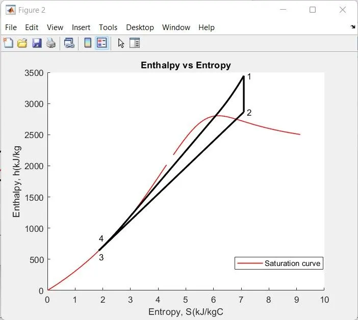
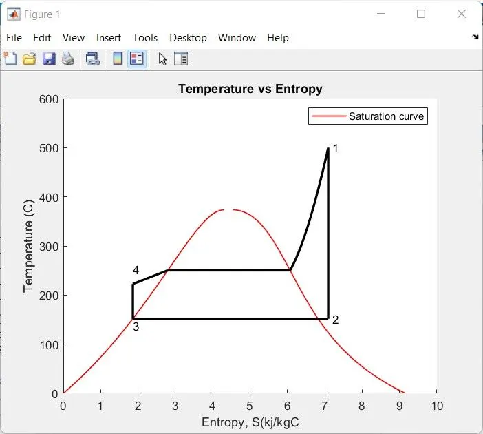
Command Window Output:

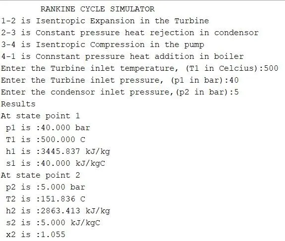
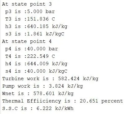
• In the above program inputs such as Turbine inlet tempertaure and pressure at state point 1 and condensor inlet pressure at state point 2 are provided.
• Xsteam library consists of steam table data for water.
• Using the XSteam function data all the state points are obtained
• sf, sg, hf, hg are calculated f stands for satured liquid and g stands for saturated vapour.
  
• Work done by turbine , pump and also heat addition into the system and heat rejection by the system and thermal efficiency are calculated by using thermodynamic relations.
• saturation curve is plotted and also with T-s and h-s plots.