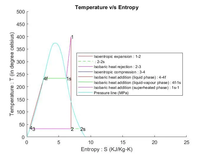
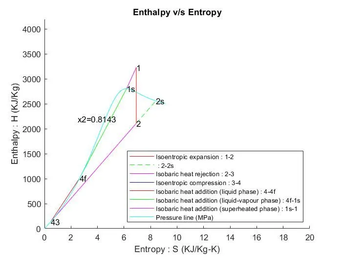
Project 2 - Rankine cycle Simulator
RANKINE CYCLE SIMULATION
OBJECTIVE:-
To learn about tools used to prepare a variation graph between two variables in the 2-D plot on Rankine cycle, which is a part of thermodynamics that allows using basic to conceptual knowledge of thermodynamics laws, concepts, formulas, properties and processes in brief.
After learning about the process details, the briefing to ‘Matlab code’ will be analysed. The pre-prepared ‘Matlab file – XSteam.m’ is used a steam-table used to find the values at given parameters.
Using this ‘XSteam.m’ file as a function to prepare code for Rankine cycle and simulate particular parameters to simulate ‘Temperature-entropy: T-S’ and ‘Enthalpy-entropy: h-s’ plot with given parameters. Find the ‘Net Work Done – Wnet’ & ‘Back Work Ratio – BWR’.
ABSTRACT:-
The Rankine Cycle is a mechanical cycle commonly used in power plants to convert the pressure energy of steam into mechanical energy through steam turbines. The Rankine Cycle’s major components include a rotating steam turbine, a boiler pump, a stationary condenser, and a boiler. A boiler is used to heat the water for steam at the required pressure and temperature as per the turbine’s requirement for power generation. The turbine exhaust is directed to the radial or axial flow condenser for condensing the steam to condensate and recycled back to the boiler through boiler pumps for heating again. This might make more sense if we take a step back, and understand what a typical cycle looks like.
Explanation of Rankine Cycle:-
The Rankine cycle is the fundamental operating cycle of all power plants where an operating fluid is continuously evaporated and condensed. The selection of operating fluid depends mainly on the available temperature range. The pressure-enthalpy (p-h), temperature-entropy (T-s) and entropy-enthalpy (h-s) are the main criteria for the evaluation or modification at any time for any process. The Rankine cycle operates in the following steps:
- 1-2 Isentropic Expansion
The vapour is expanded in the turbine, thus producing work that may be converted to electricity. In practice, the expansion is limited by the temperature of the cooling medium and by the erosion of the turbine blades by liquid entrainment in the vapour steam as the process moves further into the two-phase region. Exit vapour qualities should be greater than 90%.
- 2-3 Isobaric Heat Rejection
The vapour-liquid mixture leaving the turbine (2) is condensed at low pressure, usually in a surface condenser using cooling water. In well designed and maintained condensers, the pressure of the vapour is well below atmospheric pressure, approaching the saturation pressure of the operating fluid at the cooling water temperature.
- 3-4 Isentropic Compression
The pressure of the condensate is raised in the feed pump. Because of the low specific volume of liquids, the pump work is relatively small and often neglected in thermodynamic calculations.
- 4-1 Isobaric Heat Transfer
High-pressure liquid enters the boiler from the feed pump (3) and is heated to the saturation temperature (4). Further addition of energy causes evaporation of the liquid until it is fully converted to saturated steam (1).
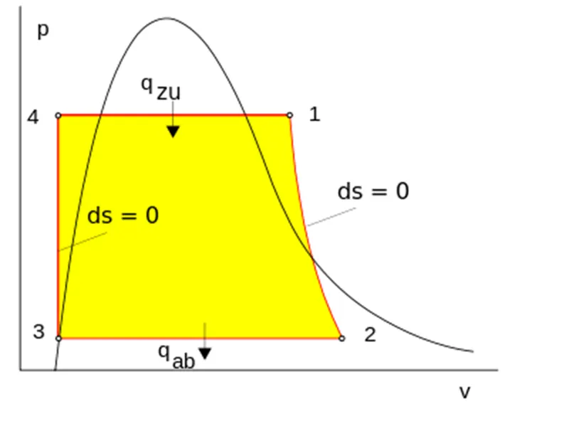
P-V Plot for Actual Rankine Cycle
The efficiency of the Ideal Rankine cycle is close to the efficiency of the Carnot cycle. But in real plants, each stage of the Rankine cycle is associated with some irreversible processes. Thus the efficiency of the Actual Rankine cycle is far lower than the Ideal Rankine cycle efficiency. Also, no heat transfer to the surroundings and no pressure loss due to mechanical moving parts are the major assumption for Ideal Rankine Cycle.
Critical Point (CP) is in the curve’s centre. The curved lines on the left side of the CP are saturated-liquid lines, and the region/area to the left of these lines are called sub-cooled liquid regions. Similarly, curved lines on the right side of the CP are saturated- vapour lines and the region/area to the right of these lines are called super-heat vapour regions.
All Rankine cycle components (boiler, turbine, condenser, and pump) are examples of a steady flow process and analysed accordingly. The energy balance for the Ideal cycle is as follows:
|
Ideal Rankine Cycle |
Heat |
Work |
|
Boiler feed pump |
Q = 0 |
Wp = h4-h3 (or) Wp = 100*vf*(P1 – P2) |
|
Boiler |
Qin = h1 – h3 |
W = 0 |
|
Turbine |
Q = 0 |
Wt = h1 – h2 |
|
Condenser |
Qout = h2 – h4 |
W = 0 |
Conceptual Thermodynamics:-
Thermodynamics is a science that deals with the relationship between heat, work, temperature and energy. The majority of laws and concept deals with the transfer of energy from ‘one point – one form’ to ‘another point – another form’. As thermodynamics defines the system properties with surroundings, to understand this first we need to know more about the system and other technical parts.
Some of these technical parts are:-
- System: A prescribed region/space or finite quantity of matter enveloped by a casing (casing is a boundary)
- Surrounding: Space & matter external to the thermodynamic system or outside the boundary
- Universe: Combination of system and surrounding
- State: The distinctive circumstances of the system at a particular point of time with described properties
- Process: The series or succession path of points through which the system passes during the transformation from one state to another state
- Cycle: The process of ongoing system through various states and returning to initial state of the system
Different types of systems in thermodynamics:-
- Closed System: No mass transfer but heat transfer take place with the system and surroundings
- Open System: Mass and heat transfer between system and surrounding
- Isolated System: No mass & no heat transfer between system and surrounding
Now few terms to know the basic of thermodynamics is studied but the various other technical properties need to be understood in quick and brief form. All the thermodynamic system at each state point is defined from only a ‘closed system’.
Process properties for the closed system:-
- Isothermal Process: - It is a constant temperature process. The heat flow into or out of the system must be slow enough to maintain thermal equilibrium. The energy entering system must leave with work.
For ideal gas, ΔT = 0 and ΔU = 0. Therefore, Q = W.
- Isochoric Process: - It is a constant volume process, when the volume of the system doesn’t change – it will do no work on its surroundings. So, W = 0 and heating gas in a closed container is an isochoric process ΔU = Q.
- Isobaric Process: - It is a constant pressure process. ΔU, W & Q are generally non-zero but calculating the work done by an ideal gas is W = P*ΔV
- Polytrophic Process: - A thermodynamic process where that obeys the relation – PVn = Constant, where ‘P: pressure’, ‘V: volume’ and ‘n: polytrophic index’. The polytrophic processes equation can describe multiple expansion & compression processes which include heat transfer. ‘Polytrophic Index’ may take value from “0 to infinity”, depending on the particular process.
- Adiabatic Process: - It is a process in which there is no exchange of heat from the system to the surrounding neither during expansion and compression, also it can either be reversible or irreversible.
Essential condition – “First”: The system must be perfectly insulated from surrounding and “Second”: Process must be carried out quickly so that there is a sufficient amount of time for heat transfer.
PVγ = Constant, where γ is ‘adiabatic index’ and is defined as the ratio of heat capacity at ‘constant pressure –cp’ to heat capacity at ‘constant volume – cv’.
- Isentropic Process: - Entropy of fluid or gas remains constant. A special adiabatic process that is reversible with no heat and matter transfer.
Since there is change in internal energy (dU) and change is volume (ΔV), so enthalpy of system is defined as:-
- H = U + P*V
- dH = dQ + V*dP
- dH =T*dS + V*dP
Entropy: It is a measure of systems thermal energy per unit temperature that is unavailable for doing useful work. Because work is obtained from ordered molecular action, the amount of entropy is also a measure of the molecular disorder or randomness of a system.
Enthalpy: It is a concept used in science & engineering when heat & work need to be calculated. When a substance changes at constant pressure, enthalpy tells how much heat & work was added or removed from the substance. Enthalpy the sum of ‘Internal energy: E’ and product of ‘Pressure: P’ & ‘Volume: V’ – “H = E + P*V”.
To determine all the above-mentioned terms and properties like heat, work, energy, enthalpy and entropy, we need to learn about the ‘Laws of Thermodynamics’.
Thermodynamic Law’s:-
- Zeroth Law: If system – A and system - B are in thermal equilibrium with system – C, then the system – A to C and system – B to C are also in thermal equilibrium.
- First Law: It is defined as the cyclic integral of heat transfer to the system being equal to the cyclic integral of work transfer to the surroundings. It is the law for ‘Conservation of Energy’, which gives a relation between heat transfers, work done and change in internal energy.
- Second Law: It induces ‘Entropy – S’ a measure of system disorder. This states that there is a natural tendency of any isolated system to degenerate into a more disordered state.
This law is explained more clearly by two statements –
- Kelvin – Plank: It is impossible to construct a device that will operate in a cycle and produce no effect other than the rising of weight and the exchange of heat with a single reservoir.
- Clausius: It is impossible to construct a device that operates in a cycle and produce no effect other than the transfer of heat from a cooler body to a hotter body.
- Third Law: It is impossible to reach a temperature of absolute zero or the entropy of a true equilibrium state of a system at T = 0K is zero.
Thermodynamic Relation & Formula:-
- Net Work Done, Wnet = Wt – Wp
- Turbine Work Done, Wt = h1 - h2
- Pump Work Done, Wp = h4 - h3 = vf3 * (P1 - P2)
- Back Work Ratio, BWR = Wp / Wt
- Heat used by turbine, Qin = h1 - h4
- Heat used by compressor, Qout = h2 - h3
- Thermal Efficiency, nth = (Wnet/Qin)*100
- Specific Steam Consumption, SSC = 3600/Wnet
- Dryness Fraction, x = (h - hf)/(hg - hf) = (s - sf)/(sg - sf)
- Sub-cooled region enthalpy, h4 = h3 + 100*vf3*(P1 - P2)
- Sub-cooled region temperature, T4 = T3*(P3/P4)^((1 - gamma)/gamma)
- gamma = cp/cv \n")
Terminology:-
- Wt: Turbine work done (KJ)
- Wp: Pump work done (KJ)
- h1: Enthalpy at state 1 - Superheated region (KJ/Kg)
- h2: Enthalpy at state 2 - Saturated region (KJ/Kg)
- h3: Enthalpy at state 3 - Saturated liquid line (KJ/Kg)
- h4: Enthalpy at state 4 - Subcooled region (KJ/Kg)
- s1: Entropy at state 1 - Superheated region (KJ/Kg-K)
- s2: Entropy at state 2 - Saturated region (KJ/Kg-K)
- s3: Entropy at state 3 - Saturated liquid line (KJ/Kg-K)
- s4: Entropy at state 4 - Subcooled region (KJ/Kg-K)
- P1: Inlet temperature of turbine (bar)
- P2: Outlet temperature of turbine (bar)
- P3: Inlet temperature of condenser (bar)
- P4: Outlet temperature of condenser (bar)
- sf: Specific entropy at saturated liquid state (KJ/Kg-K)
- sg: Specific entropy at saturated vapour state (KJ/Kg-K)
- hf: Specific enthalpy at saturated liquid state (KJ/Kg)
- hg: Specific enthalpy at saturated vapour state (KJ/Kg)
- hfg: Latent heat of vaporization (KJ/Kg)
- vf3: Specific volume at saturated vapour state (m^3/Kg)
- x: Dryness fraction
- T1: Superheated temperature (degree Celsius)
- T2: Saturation temperature at pressure 2 (degree Celsius)
- T3: Saturation temperature at pressure 2 (degree Celsius)
- T4: Saturation temperature in the subcooled region (degree Celsius)
- cp: Specific heat at constant pressure (KJ/Kg-K)
- cv: Specific heat at constant volume (KJ/Kg-K)
UNDERSTANDING OF “XSteam.m”:
- Code can be written in two formats:-
- XSteam(‘h_pt’,p,t) :- Returns the enthalpy value at p bar & t deg. C
- XSteam(‘Tsat_p,p) :- Returns the saturation temp. at p bar
- This file is a function that needs to be called with proper case-sensitive parameters
- Whenever the function is called out proper syntax of calling is needed
- To define and find parameters of the Rankine cycle we need these functions to be called out:-
- Temperature
- Enthalpy
- Entropy
- Specific volume
- Specific isobaric heat capacity
- Specific isochoric heat capacity
- All these values need at least one parameter, which can either be pressure or temperature or both pressure & temperature
EXPLANATION OF CODE:
- First 85 line describe about the Rankine cycle with help of “fprintf”. These include the Objective, Formulas, Terminologies and user Input value
- Input values: P1, P2 and T1
- Using thermodynamic relation, value for P4 and P3 is obtained
- Using ‘XSteam’ saturation temperature at pressure 1 is obtained
- Using ‘XSteam’ state 1 - entropy at pressure & temperature of state 1 is obtained
- Using ‘XSteam’ state 3 - entropy at pressure 3 is obtained
- By Isentropic expansion, s2 = s1
- By Isentropic compression, s4 = s3
- All specific values of enthalpy & entropy are calculated using ‘XSteam’
- Using ‘XSteam’ saturation temperature at pressure 2, state 2 - temperature is obtained
- By Isothermal compression, T3 = T2
- Using thermodynamic relation value of T4 is obtained, T4 = T3*(P4/P3)^((gamma - 1)/gamma)
- In above gamma = cp4/cv4 and cp & cv is calculated from ‘XSteam’
- Using ‘XSteam’ state 1 - enthalpy at pressure & temperature of state 1 is obtained
- Using ‘XSteam’ state 3 - enthalpy at pressure 3 is obtained
- Using thermodynamic relation value of h2 is obtained, h2 = hf2 + x2*(hg2 - hf2)
- And dryness fraction, x2 = (s2 - sf2)/(sg2 - sf2)
- Using thermodynamic relation value of h4 is obtained, h4 = h3 + 100*vf3*(P1 - P2)
- And Specific volume, vf3 = XSteam('vl_p',P3)
- After all these parameters are obtained, calculation of output will be done –
- Wt = h1 - h2
- Wp = h4 - h3
- Wnet = Wt - Wp
- BWR = Wp/Wt
- Qin = h1 - h4
- Qout = h2 - h3
- nth = (Wnet/Qin)*100
- SSC = 3600/Wnet
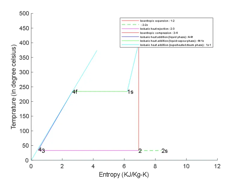
- Now to create a saturation curve the iterated base value is needed and for that ‘temperature’ the best source is chosen. Using the ‘linspace’ command, the temperature is given a value range of (0,374) with 500 iterations. All these iterations are the coordinates at various sub-state of the Rankine cycle.
- As the Entropy & Enthalpy are defined with the values w.r.t. temperature range (T), these values will now be calculated again with iteration same as of temperature in the loop.
- To create a plot we will use all the above-defined values of pressure, temperature, entropy & enthalpy. But for the saturation curve, we will use only iterated values of any state.
- Two figures need to be created, so they will be categorized with “figure -1” & “figure – 2”. For both the figures, we will have to use the same methodology.
- To create a plot, first, we will use the ‘hold on’ command to store all data without executing them.
- Then for every state point, the plot will be created.
- To view the plot in the proper way we will use the ‘axis’ command to define the plot area.
- To specify all the items in the plot we will use title, xlabel, ylabel & legend.
- After all plot commands are written we will execute them by using the ‘hold off’ command.
- At last, have to print all the values of their specific region and output values.
ERRORS OCCURRED DURING CODING: -
- The printing command ‘fprintf’ is coded wrong ‘fpritf’.
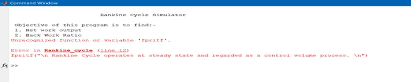
Correction – All printing commands are corrected to ‘fprintf’.
- Incorrect calling of function.
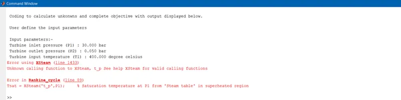
Correction – This is the most crucial part of coding, calling the “XSteam.m” function for particular values at a particular state. To execute this command correctly, the ‘XSteam’ file need attention to it in a more careful manner. All the particulars in the file are ‘case-sensitive’, so this encryption makes it more difficult to code but after a few looks on the file it becomes more familiar.
All the state points are defined with particular pre-defined nomenclature but these need the attention of input with correct properties as required by that state. For example, at state 1 the value of ‘entropy’ needs both values of temperature & pressure as it is in the superheated region. So this kind of understanding is needed to identify the real values to be written while coding.
- Incorrect inputs while plotting T-S graph
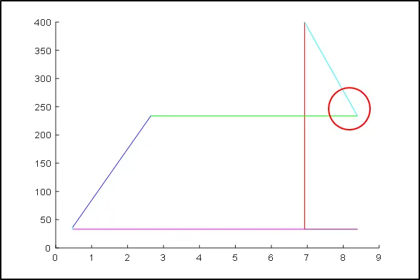
Here the red marked area is given incorrect input. The value is defined with state 2s.
Correction – The defined value here is of state ‘2s’ is ‘specific entropy at the saturated region in vapour phase’ but this input is incorrect. After analysing the plot the input value is changed to ‘1s’ which is ‘specific entropy at superheated region’. After using the ‘1s’ value the plot obtained is the true T-S plot.
- Incorrect inputs while plotting H-S graph
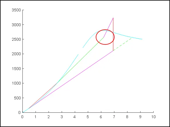
Here the red marked area is given incorrect input. The value is defined with state 2s.
plot([sf4 sg1],[hf4 hg2],'color','g')
plot([sg1 s1],[hg2 h1],'color','m')
Correction – The defined value here is of state ‘2s’ is ‘specific entropy at saturated region in vapour phase’ but this input is incorrect. After analysing the plot the input value is changed to ‘1s’ which is ‘specific entropy at superheated region’. After using ‘1s’ value the plot obtained is the true T-S plot.
plot([sf4 sg1],[hf4 hg4],'color','g')
plot([sg1 s1],[hg4 h1],'color','m')
- Incorrect coordinates for saturation line
Coding to plot saturation curve:
T = linspace(0,374,500);
s = XSteam('sl_T',373);
sf = linspace(0,s,500);
sg = linspace(0,XSteam('sv_T',374),500);
Correction – The code above has no logic to implement a curvature with specified coordinates. So this is eliminated and proper logical coding is done.
T = linspace(0,374,500);
sf = zeros;
sg = zeros;
hf = zeros;
hg = zeros;
for i = 1:length(T)
sf(i) = XSteam('sl_T',T(i))
sg(i) = XSteam('sv_T',T(i))
hf(i) = XSteam('hl_T',T(i))
hg(i) = XSteam('hv_T',T(i))
end
After using this logical code we have obtained a proper set of coordinates to plot the saturation curve for both T-S and H-S plots in a specified way.
REFERENCES:-
- https://www.electrical4u.com/ideal-verses-actual-in-rankine-cycle/
- https://thermopedia.com/content/1072/
- https://energyeducation.ca/encyclopedia/Rankine_cycle
- Book: Engineering Thermodynamics – P.K. Nag
- Book: Thermodynamics – Cengel & Boles
- https://in.mathworks.com/help/matlab/ref/axis.html
- https://in.mathworks.com/help/matlab/ref/text.html
- https://in.mathworks.com/help/matlab/ref/xlabel.html
- https://in.mathworks.com/help/matlab/ref/ylabel.html
- https://in.mathworks.com/help/matlab/ref/title.html
- https://in.mathworks.com/help/matlab/ref/figure.html
- https://in.mathworks.com/help/matlab/ref/legend.html
- https://in.mathworks.com/help/matlab/ref/hold.html
MAIN CODE:
clear all
close all
clc

fprintf("\n                        Rankine Cycle Simulator \n")

fprintf("\n Objective of this program is to find:-")
fprintf("\n 1. Net work output")
fprintf("\n 2. Back Work Ratio \n")

% Explanation of Rankine cycle process
fprintf("\n Rankine Cycle operates at steady state and regarded as a control volume process. \n")
fprintf(" Four basic cycles of Rankine cycle:- \n")
fprintf(" Cycle 1-2 : Isoentropic Expansion (Reversible adiabatic expansion of steam in steam turbine \n")
fprintf(" Cycle 2-3 : Constant Pressure Heat Rejection (Constant pressure heat rejection in the condensor to convert condensate into water \n")
fprintf(" Cycle 3-4 : Isoentropic Compression (Reversible adiabatic condensation from pump to boiler \n")
fprintf(" Cycle 4-1 : Constant Pressure Heat Addition (Water to steam by heat addition in boiler \n")

% Formulas used to calculate unknowns in Rankine cycle process
fprintf(" \n Unknowns and their formulas:- \n")
fprintf(" * Wnet = Wt - Wp                  : Net Work Output \n")
fprintf(" * Wt = h1 - h2                    : Turbine work done \n")
fprintf(" * Wp = h4 - h3 = vf3 * (P1 - P2)  : Pump work done \n")
fprintf(" * BWR = Wp / Wt                   : Back Work Ratio \n")
fprintf(" * Qin = h1 - h4                   : Heat used by turbine \n")
fprintf(" * Qout = h2 - h3                  : Heat released by compressor \n")
fprintf(" * nth = (Wnet/Qin)*100            : Thermal efficiency of cycle \n")
fprintf(" * SSC = 3600/Wnet                 : Specific steam consumption \n")
fprintf(" * h1 = hg + cps*(T1 - Tsat)       : Superheated region \n")
fprintf(" * s1 = sg + cps*ln(T1/Tsat)       : Superheated region \n")
fprintf(" * h2 = hf                         : Saturated region \n")
fprintf(" * h3 = hf + x*hfg                 : Saturated liquid line \n")
fprintf(" * s3 = sf + x*sfg                 : Saturated liquid line \n")
fprintf(" * h4 = h3 + 100*vf3*(P1 - P2)     : Subcooled region \n")
fprintf(" * hfg = hg - hf \n")
fprintf(" * sfg = sg - sf \n")
fprintf(" * x = (h - hf)/(hg - hf) = (s - sf)/(sg - sf) \n")
fprintf(" * P3 = P2 and P4 = P1 \n")
fprintf(" * T2 = T3 = Tsat                  : Saturation temperature \n")
fprintf(" * T4 = T3*(P3/P4)^((1 - gamma)/gamma) \n")
fprintf(" * gamma = cp/cv \n")

% Terminology used in Rankine cycle process
fprintf(" \n Terminology:- \n")
fprintf(" * Wt  : Turbine work done (KJ) \n")
fprintf(" * Wp  : Pump work done (KJ) \n")
fprintf(" * h1  : Enthalpy at state 1 - Superheated region (KJ/Kg) \n")
fprintf(" * h2  : Enthalpy at state 2 - Saturated region (KJ/Kg) \n")
fprintf(" * h3  : Enthalpy at state 3 - Saturated liquid line (KJ/Kg) \n")
fprintf(" * h4  : Enthalpy at state 4 - Subcooled region (KJ/Kg) \n")
fprintf(" * s1  : Entropy at state 1 - Superheated region (KJ/Kg-K)\n")
fprintf(" * s2  : Entropy at state 2 - Saturated region (KJ/Kg-K) \n")
fprintf(" * s3  : Entropy at state 3 - Saturated liquid line (KJ/Kg-K) \n")
fprintf(" * s4  : Entropy at state 4 - Subcooled region (KJ/Kg-K) \n")
fprintf(" * P1  : Inlet temperature of turbine (bar) \n")
fprintf(" * P2  : Outlet temperature of turbine (bar) \n")
fprintf(" * P3  : Inlet temperature of condenser (bar) \n")
fprintf(" * P4  : Outlet temperature of condenser (bar) \n")
fprintf(" * sf  : Specific entropy at saturated liquid state (KJ/Kg-K) \n")
fprintf(" * sg  : Specific entropy at saturated vapour state (KJ/Kg-K) \n")
fprintf(" * hf  : Specific enthalpy at saturated liquid state (KJ/Kg) \n")
fprintf(" * hg  : Specific enthalpy at saturated vapour state (KJ/Kg) \n")
fprintf(" * hfg : Latent heat of vaporization (KJ/Kg) \n")
fprintf(" * vf3 : Specific volume at saturated vapour state (m^3/Kg) \n")
fprintf(" * x   : Dryness fraction \n")
fprintf(" * T1  : Superheated temperature (degree Celsius) \n")
fprintf(" * T2  : Saturation temperature at pressure 2 (degree Celsius) \n")
fprintf(" * T3  : Saturation temperature at pressure 2 (degree Celscius) \n")
fprintf(" * T4  : Saturation temperature in subcooled region (degree Celsius) \n")
fprintf(" * cp  : Specific heat at constant pressure (KJ/Kg-K) \n")
fprintf(" * cv  : Specific heat at constant volume (KJ/Kg-K) \n")

% Coding for the calculation of all unknowns to complete the objective :
fprintf("\n Coding to calculate unknowns and complete objective with output displayed below. \n")

% Given parameters (User defined parameter)
fprintf(" \n User define the input parameters \n\n")
P1 = 30;                        % Turbine inlet pressure (bar)
T1 = 400;                       % Turbine input temperature (degree celsius)
P2 = 0.05;                      % Condensor inlet pressure (bar)
fprintf(" Input parameters:- \n")
fprintf(" Turbine inlet pressure (P1) : %0.3f bar\n",P1)
fprintf(" Turbine outlet pressure (P2) : %0.3f bar\n",P2)
fprintf(" Turbine input temperature (T1) : %0.3f degree celsius\n",T1)

% Pressure relation obtained from Rankine cycle process
P4 = P1;                        % Isothermal expansion : heat is added from state 4 to sate 1 from P-V diagram
P3 = P2;                        % Isobaric compression : heat is rejected from state 2 to state 3 from P-V diagram
Tsat = XSteam('tsat_p',P1);     % Saturation temperature at P1 from 'Steam table' in superheated region

% Entropy calculation at different state point
s1 = XSteam('s_pT',P1,T1);      % Entropy of superheated steam from 'Steam table'
s2 = s1;                        % Isoentropic expansion : expansion of adiabatic reversible steam in turbine
s3 = XSteam('sl_p',P3);         % Entropy of saturated steam from 'Steam table'
s4 = s3;                        % Isoentropic compression : compression of adiabatic reversible steam from pump to boiler

% Specific entropy and enthalpy values at different state point-Steam table
hf1 = XSteam('hl_T',Tsat);      % Specific enthalpy at superheated region in liquid phase
sg1 = XSteam('sv_T',Tsat);      % Specific entropy at superheated region in vapour phase
hf2 = XSteam('hl_p',P2);        % Specific enthalpy at saturated region in fluid phase
hg2 = XSteam('hv_p',P2);        % Specific enthalpy at saturated region in vapour phase
sf2 = XSteam('sl_p',P2);        % Specific entropy at saturated region in fluid phase
sg2 = XSteam('sv_p',P2);        % Specific entropy at saturated region in vapour phase
hf4 = XSteam('hl_p',P4);        % Specific enthalpy at liquid region in liquid phase
sf4 = XSteam('sl_p',P4);        % Specific entropy at liquid region in liquid phase
hg4 = XSteam('hv_p',P4);        % Specific enthalpy at liquid region in vapour phase
sg4 = XSteam('sv_p',P4);        % Specific entropy at liquid region in vapour phase

% temperature's obtained from steam table "XSteam.m"
T2 = XSteam('tsat_p',P2);       % Saturation temperature at P2 will give state 2 temperature
T3 = T2;                        % Isothermal compression : same temperature in both state from T-S diagram
% T4 can only be found by using thermodynamic relation : T4 = T3*(P4/P3)^((gamma - 1)/gamma)
cp4 = XSteam('cp_ps',P4,s4);    % Specific heat of liquid region at constant pressure
cv4 = XSteam('cv_ps',P4,s4);    % Specific heat of liquid region at constant volume
gamma = cp4/cv4;                % Adiabatic constant : Ratio of Cp and Cv
T4 = T3*(P4/P3)^((gamma - 1)/gamma);

% Enthalpy calculation at different state point
h1 = XSteam('h_pT',P1,T1);      % Enthalpy of superheated steam from 'Steam table' with pressure & temperature as a function
x2 = (s2 - sf2)/(sg2 - sf2);    % Dryness fraction : Ratio of dry steam to mixture of steam
h2 = hf2 + x2*(hg2 - hf2);      % Enthalpy of saturated steam from thermodynamic relation
h3 = XSteam('hl_p',P3);         % Enthalpy of steam at liquid line from 'Steam table' with pressure as a function
vf3 = XSteam('vl_p',P3);        % Specific volume of steam at liquid phase in liquid line region
h4 = h3 + 100*vf3*(P1 - P2);    % Enthalpy of steam in liquid region from thermodynamic relation

% Output calculation for objective from parameters obtained at different states
% Objectives and related outputs are calculated from thermodynamic relations

Wt = h1 - h2;                   % Work done by turbine
Wp = h4 - h3;                   % Work done by pump
Wnet = Wt - Wp;                 % Net work done of cycle
BWR = Wp/Wt;                    % Back Work Ratio
% BWR is ratio of compressor work to turbine work
% Other parameters that can be calculated from these above parameters
Qin = h1 - h4;                  % Heat used by turbine
Qout = h2 - h3;                 % Heat released by compressor
nth = (Wnet/Qin)*100;           % Thermal efficiency of single cycle
SSC = 3600/Wnet;                % Specific steam consumption (SSC)
% SSC is amount of steam required to produce unit work

% Plot for T-S and H-S with different calculated state points
% Pressure line in both diagram can only plotted with looped iterations
% Iteration w.r.t. temperature is done, not to make programming complex
% 'linspace' with 500 iteration is used for defining temperature range
T = linspace(0,374,500);
sf = zeros;                         % Preallocation provided to avoid error while loop
sg = zeros;                         % Preallocation provided to avoid error while loop
hf = zeros;                         % Preallocation provided to avoid error while loop
hg = zeros;                         % Preallocation provided to avoid error while loop
% 'for' loop is used to allocate single function to different variables
for i = 1:length(T)                 % temperature is defined as largest dimensioned array 'length'
    sf(i) = XSteam('sl_T',T(i));    % Specific liquid entropy as a function of iterated temperature
    sg(i) = XSteam('sv_T',T(i));    % Specific vapour entropy as a function of iterated temperature
    hf(i) = XSteam('hl_T',T(i));    % Specific liquid enthalpy as a function of iterated temperature
    hg(i) = XSteam('hv_T',T(i));    % Specific vapour entahlpy as a function of iterated temperature
end

% Plotting T-S diagram:-
figure(1)                           % Allocation done when no. of 'figure' need to be created
hold on                             % used to execute all commands simultaneously and hold the process until steps are completed

% 'plot' used to graph between two points with simplicity and ease
% plot(x,y,'linestyle/lineweight/color/etc') can be used to define graph
plot([s1 s2],[T1 T2],'color','r')
plot([s2 sg2],[T2 T2],'linestyle','--','color','g')
plot([s2 s3],[T2 T3],'color','m')
plot([s3 s4],[T3 T4],'color','b')
plot([s4 sf4],[T4 Tsat],'color','r')
plot([sf4 sg1],[Tsat Tsat],'color','g')
plot([sg1 s1],[Tsat T1],'color','m')
plot(sf,T,'color','c')
plot(sg,T,'color','c')
plot([4.257 4.603],[373.3 373.3],'color','c')
% axis is used to define the spacework for plotting the graph
axis([0 15 0 500])

% text used to specify or highlight key point in plotted graph
% text(x,y,text,'textstyle/fontsize/color/etc') define text in graph
text(s1,T1,'1','fontsize',10)
text(s2,T2,'2','fontsize',10)
text(s3,T3,'  3','fontsize',10)
text(s4,T4,'4','fontsize',10)
text(sg2,T2,'2s','fontsize',10)
text(sf4,Tsat,'4f','fontsize',10)
text(sg1,Tsat,'1s','fontsize',10)
text(4,400,'x2=0.8143','fontsize',10)

% title decribe the plot
title(" Temperature v/s Entropy ")
% xlabel defines the x-axis plot
xlabel('Entropy : S (KJ/Kg-K)')
% ylabel defines the y-axis plot
ylabel('Temperature : T (in degree celsius)')
% legend is used to elaborate the labels in descriptive way of various plot
legend('Isoentropic expansion : 1-2',' : 2-2s','Isobaric heat rejection : 2-3','Isoentropic compression : 3-4','Isobaric heat addition (liquid phase) : 4-4f','Isobaric heat addition (liquid-vapour phase) : 4f-1s','Isobaric heat addition (superheated phase) : 1s-1','Pressure line (MPa)','fontsize',5)

hold off                            % close the ongoing process and save it

% Plotting H-S diagram:-
figure(3)                           % Allocation done when no. of 'figure' need to be created
hold on                             % used to execute all commands simultaneously and hold the process until steps are completed

% 'plot' used to graph between two points with simplicity and ease
% plot(x,y,'linestyle/lineweight/color/etc') can be used to define graph
plot([s1 s2],[h1 h2],'color','r')
plot([s2 sg2],[h2 hg2],'linestyle','--','color','g')
plot([s2 s3],[h2 h3],'color','m')
plot([s3 s4],[h3 h4],'color','b')
plot([s4 sf4],[h4 hf4],'color','r')
plot([sf4 sg1],[hf4 hg4],'color','g')
plot([sg1 s1],[hg4 h1],'color','m')
plot(sf,hf,'color','c')
plot(sg,hg,'color','c')
plot([4.257 4.603],[1987 2211],'color','c')
% axis is used to define the spacework for plotting the graph
axis([0 15 0 3800])

% text used to specify or highlight key point in plotted graph
% text(x,y,text,'textstyle/fontsize/color/etc') define text in graph
text(s1,h1,'1','fontsize',10)
text(s2,h2,'2','fontsize',10)
text(s3,h3,'  3','fontsize',10)
text(s4,h4,'4','fontsize',10)
text(sg2,hg2,'2s','fontsize',10)
text(sf4,hf4,'4f','fontsize',10)
text(sg1,hg4,'1s','fontsize',10)
text(2.5,2200,'x2=0.8143','fontsize',10)

% title defines the plot
title(" Enthalpy v/s Entropy ")
% xlabel defines the x-axis plot
xlabel('Entropy : S (KJ/Kg-K)')
% xlabel defines the y-axis plot
ylabel('Enthalpy : H (KJ/Kg)')
% legend is used to elaborate the labels in descriptive way of various plot
legend('Isoentropic expansion : 1-2',' : 2-2s','Isobaric heat rejection : 2-3','Isoentropic compression : 3-4','Isobaric heat addition (liquid phase) : 4-4f','Isobaric heat addition (liquid-vapour phase) : 4f-1s','Isobaric heat addition (superheated phase) : 1s-1','Pressure line (MPa)','fontsize',5)

hold off                            % close the ongoing process and save it

% Coding is executed for all variables, parameters and plots

% Printing of obtained values w.r.t. their region

% Printing specific entities value
fprintf("\n Value of specific entities:- \n")
fprintf("\n     * Specific heat (pressure constant) in liquid region, cp4 = %0.3f",cp4)
fprintf("\n     * Specific heat (volume constant) in liquid region, cv4 = %0.3f",cv4)
fprintf("\n     * Specific fluid enthalpy (superheated region), hf1 = %0.3f KJ/Kg",hf1)
fprintf("\n     * Specific vapour entropy (superheated region), sg1 = %0.3f KJ/Kg-K",sg1)
fprintf("\n     * Specific fluid enthalpy (saturated region), hf2 = %0.3f KJ/Kg",hf2)
fprintf("\n     * Specific vapour enthalpy (saturated region), hg2 = %0.3f KJ/Kg",hg2)
fprintf("\n     * Specific fluid entropy (saturated region), sf2 = %0.3f KJ/Kg-K",sf2)
fprintf("\n     * Specific vapour entropy (saturated region), sg2 = %0.3f KJ/Kg-K",sg2)
fprintf("\n     * Specific fluid enthalpy (liquid region), hf4 = %0.3f KJ/Kg",hf4)
fprintf("\n     * Specific vapour enthalpy (liquid region), hg4 = %0.3f KJ/Kg",hg4)
fprintf("\n     * Specific fluid entropy (liquid region), sf4 = %0.3f KJ/Kg-K",sf4)
fprintf("\n     * Specific vapour entropy (liquid region), sg4 = %0.3f KJ/Kg-K \n",sg4)

% Printing values of state 1
fprintf("\n Region 1 - Superheated steam region:- \n")
fprintf("\n     * Input pressure, P1 = %0.3f bar",P1)
fprintf("\n     * Input temperature, T1 = %0.3f degree celsius",T1)
fprintf("\n     * Enthalpy of superheated steam, h1 = %0.3f KJ/kg",h1)
fprintf("\n     * Entropy of superheated steam, s1 = %0.3f KJ/Kg-K",s1)
fprintf("\n     * Saturation temperature (at pressure 1), Tsat = %0.3f degree celsius \n",Tsat)

% Printing values of state 2
fprintf("\n Region 2 - Saturated steam region:- \n")
fprintf("\n     * Input pressure, P2 = %0.3f bar",P2)
fprintf("\n     * Saturation temperature (at pressure 2), T2 = %0.3f degree celsius",T2)
fprintf("\n     * Enthalpy of saturated steam, h2 = %0.3f KJ/kg",h2)
fprintf("\n     * Entropy of superheated steam, s2 = %0.3f KJ/Kg-K",s2)
fprintf("\n     * Dryness fraction, x2 = %0.3f \n",x2)

% Printing values of state 3
fprintf("\n Region 3 - Saturated liquid line region:- \n")
fprintf("\n     * Saturation region pressure, P3 = %0.3f bar",P3)
fprintf("\n     * Saturation temperature (at pressure 2), T3 = %0.3f degree celsius",T3)
fprintf("\n     * Enthalpy of wet steam, h3 = %0.3f KJ/kg",h3)
fprintf("\n     * Entropy of saturated steam, s3 = %0.3f KJ/Kg-K \n",s3)

% Printing values of state 4
fprintf("\n Region 4 - Liquid region:- \n")
fprintf("\n     * Wet steam pressure, P4 = %0.3f bar",P4)
fprintf("\n     * Wet steam temperature, T4 = %0.3f degree celsius",T4)
fprintf("\n     * Enthalpy of condensed steam, h4 = %0.3f KJ/kg",h4)
fprintf("\n     * Entropy of saturated steam, s4 = %0.3f KJ/Kg-K \n",s4)

% Printing output values
fprintf("\n Obtained outputs:- \n")
fprintf("\n   * Turbine work done, Wt = %0.3f KJ/Kg",Wt)
fprintf("\n   * Pump work done, Wp = %0.3f KJ/Kg",Wp)
fprintf("\n   * Net work done, Wnet = %0.3f KJ/Kg",Wnet)
fprintf("\n   * Back work ratio, BWR = %0.5f",BWR)
fprintf("\n   * Heat useds by turbine, Qin = %0.3f KJ/Kg",Qin)
fprintf("\n   * Heat released by condensor, Qout = %0.3f KJ/Kg",Qout)
fprintf("\n   * Thermal efficiency of cycle, nth = %0.3f",nth)
fprintf("\n   * Specific steam consumption, SSC = %0.3f Kg/KJ\n",SSC)
COMMAND WINDOW:
                        Rankine Cycle Simulator

 The objective of this program is to find:-
 1. Net work output
 2. Back Work Ratio

 Rankine Cycle operates at a steady state and is regarded as a control volume process.
 Four basic cycles of Rankine cycle:-
 Cycle 1-2: Isoentropic Expansion (Reversible adiabatic expansion of steam in steam turbine
 Cycle 2-3: Constant Pressure Heat Rejection (Constant pressure heat rejection in the condenser to convert condensate into water
 Cycle 3-4: Isoentropic Compression (Reversible adiabatic condensation from the pump to boiler
 Cycle 4-1: Constant Pressure Heat Addition (Water to steam by heat addition in the boiler

 Unknowns and their formulas:-
 * Wnet = Wt - Wp                  : Net Work Output
 * Wt = h1 - h2                    : Turbine work done
 * Wp = h4 - h3 = vf3 * (P1 - P2)  : Pump work done
 * BWR = Wp / Wt                   : Back Work Ratio
 * Qin = h1 - h4                   : Heat used by turbine
 * Qout = h2 - h3                  : Heat released by compressor
 * nth = (Wnet/Qin)*100            : Thermal efficiency of cycle
 * SSC = 3600/Wnet                 : Specific steam consumption
 * h1 = hg + cps*(T1 - Tsat)       : Superheated region
 * s1 = sg + cps*ln(T1/Tsat)       : Superheated region
 * h2 = hf                         : Saturated region
 * h3 = hf + x*hfg                 : Saturated liquid line
 * s3 = sf + x*sfg                 : Saturated liquid line
 * h4 = h3 + 100*vf3*(P1 - P2)     : Subcooled region
 * hfg = hg - hf
 * sfg = sg - sf
 * x = (h - hf)/(hg - hf) = (s - sf)/(sg - sf)
 * P3 = P2 and P4 = P1
 * T2 = T3 = Tsat                  : Saturation temperature
 * T4 = T3*(P3/P4)^((1 - gamma)/gamma)
 * gamma = cp/cv

 Terminology:-
 * Wt  : Turbine work done (KJ)
 * Wp  : Pump work done (KJ)
 * h1  : Enthalpy at state 1 - Superheated region (KJ/Kg)
 * h2  : Enthalpy at state 2 - Saturated region (KJ/Kg)
 * h3  : Enthalpy at state 3 - Saturated liquid line (KJ/Kg)
 * h4  : Enthalpy at state 4 - Subcooled region (KJ/Kg)
 * s1  : Entropy at state 1 - Superheated region (KJ/Kg-K)
 * s2  : Entropy at state 2 - Saturated region (KJ/Kg-K)
 * s3  : Entropy at state 3 - Saturated liquid line (KJ/Kg-K)
 * s4  : Entropy at state 4 - Subcooled region (KJ/Kg-K)
 * P1  : Inlet temperature of turbine (bar)
 * P2  : Outlet temperature of turbine (bar)
 * P3  : Inlet temperature of condenser (bar)
 * P4  : Outlet temperature of condenser (bar)
 * sf  : Specific entropy at saturated liquid state (KJ/Kg-K)
 * sg  : Specific entropy at saturated vapour state (KJ/Kg-K)
 * hf  : Specific enthalpy at saturated liquid state (KJ/Kg)
 * hg  : Specific enthalpy at saturated vapour state (KJ/Kg)
 * hfg : Latent heat of vaporization (KJ/Kg)
 * vf3 : Specific volume at saturated vapour state (m^3/Kg)
 * x   : Dryness fraction
 * T1  : Superheated temperature (degree Celsius)
 * T2  : Saturation temperature at pressure 2 (degree Celsius)
 * T3  : Saturation temperature at pressure 2 (degree Celscius)
 * T4  : Saturation temperature in subcooled region (degree Celsius)
 * cp  : Specific heat at constant pressure (KJ/Kg-K)
 * cv  : Specific heat at constant volume (KJ/Kg-K)

 Coding to calculate unknowns and complete objective with output displayed below.

 User define the input parameters

 Input parameters:-
 Turbine inlet pressure (P1): 30.000 bar
 Turbine outlet pressure (P2): 0.050 bar
 Turbine input temperature (T1): 400.000 degree celsius

 Value of specific entities:-

     * Specific heat (pressure constant) in liquid region, cp4 = 4.172
     * Specific heat (volume constant) in liquid region, cv4 = 4.096
     * Specific fluid enthalpy (superheated region), hf1 = 1008.371 KJ/Kg
     * Specific vapour entropy (superheated region), sg1 = 6.186 KJ/Kg-K
     * Specific fluid enthalpy (saturated region), hf2 = 137.765 KJ/Kg
     * Specific vapour enthalpy (saturated region), hg2 = 2560.765 KJ/Kg
     * Specific fluid entropy (saturated region), sf2 = 0.476 KJ/Kg-K
     * Specific vapour entropy (saturated region), sg2 = 8.394 KJ/Kg-K
     * Specific fluid enthalpy (liquid region), hf4 = 1008.371 KJ/Kg
     * Specific vapour enthalpy (liquid region), hg4 = 2803.265 KJ/Kg
     * Specific fluid entropy (liquid region), sf4 = 2.646 KJ/Kg-K
     * Specific vapour entropy (liquid region), sg4 = 6.186 KJ/Kg-K

 Region 1 - Superheated steam region:-

     * Input pressure, P1 = 30.000 bar
     * Input temperature, T1 = 400.000 degree celsius
     * Enthalpy of superheated steam, h1 = 3231.571 KJ/kg
     * Entropy of superheated steam, s1 = 6.923 KJ/Kg-K
     * Saturation temperature (at pressure 1), Tsat = 233.858 degree celsius

 Region 2 - Saturated steam region:-

     * Input pressure, P2 = 0.050 bar
     * Saturation temperature (at pressure 2), T2 = 32.875 degree celsius
     * Enthalpy of saturated steam, h2 = 2110.708 KJ/kg
     * Entropy of superheated steam, s2 = 6.923 KJ/Kg-K
     * Dryness fraction, x2 = 0.814

 Region 3 - Saturated liquid line region:-

     * Saturation region pressure, P3 = 0.050 bar
     * Saturation temperature (at pressure 2), T3 = 32.875 degree celsius
     * Enthalpy of wet steam, h3 = 137.765 KJ/kg
     * Entropy of saturated steam, s3 = 0.476 KJ/Kg-K

 Region 4 - Liquid region:-

     * Wet steam pressure, P4 = 30.000 bar
     * Wet steam temperature, T4 = 36.935 degree celsius
     * Enthalpy of condensed steam, h4 = 140.776 KJ/kg
     * Entropy of saturated steam, s4 = 0.476 KJ/Kg-K

 Obtained outputs:-

   * Turbine work done, Wt = 1120.863 KJ/Kg
   * Pump work done, Wp = 3.011 KJ/Kg
   * Net work done, Wnet = 1117.852 KJ/Kg
   * Back work ratio, BWR = 0.00269
   * Heat useds by turbine, Qin = 3090.795 KJ/Kg
   * Heat released by condensor, Qout = 1972.943 KJ/Kg
   * Thermal efficiency of cycle, nth = 36.167
   * Specific steam consumption, SSC = 3.220 Kg/KJ
>>
PLOTS: