Project 2 - Rankine cycle Simulator
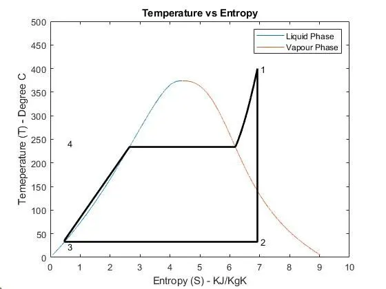
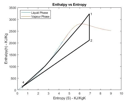
AIM: To create a Rankine Cycle Simulator using OCTAVE/MATLAB & calculate the state points of the Rankine Cycle (any type of your choice) based on user inputs. Plot the corresponding T-s and h-s plots for the given set of inputs.
ABOUT:
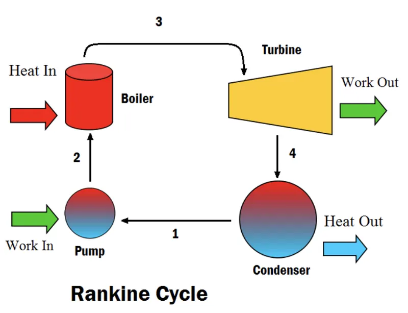
The Rankine cycle or Rankine Vapor Cycle is the process widely used by power plants such as coal power plants or . In this mechanism, a fuel is used to produce heat within a boiler, converting water into steam which then expands through a turbine producing useful work. This process was developed in 1859 by Scottish engineer William J.M. Rankine. This is a thermodynamic cycle which converts heat into mechanical energy—which usually gets transformed into electrical.
- Pump: Compression of the fluid to high pressure using a pump.
- Boiler: The compressed fluid is heated to the final temperature (which is at boiling point), therefore, a phase change occurs—from liquid to vapor.
- Turbine: Expansion of the vapor in the turbine.
- Condenser: Condensation of the vapor in the condenser.
The efficiency of the Rankine cycle is limited by the high heat of vaporization by the fluid. The fluid must be cycled through and reused constantly, therefore, water is the most practical fluid for this cycle. This is not why many power plants are located near a body of water—that's for the waste heat.
As the water condenses in the condenser, waste heat is given off in the form of water vapour—which can be seen billowing from a plant's cooling towers. This waste heat is necessary in any thermodynamic cycle. Due to this condensation step, the pressure at the turbine outlet is lowered. This means the pump requires less work to compress the water—resulting in higher overall efficiencies.
CODE:
% RANKINE CYCLE SIMULATOR
clear all
close all
clc

disp('Rankine Cycle Simulator')
disp('Process 1-2: Isentropic expansion in turbine')
disp('Process 2-3: Constant Pressure Heat Rejection in Condenser')
disp('Process 3-4: Isentropic Compression in Pump')
disp('Process 4-1: Constant Pressure Heat Addition in Boiler')

% Initial data Inputs ; Directly give the values of T1, P1 & P2
T1 = input('Turbine Inlet Temperature (Deg C) = ');
p1 = input('Turbine Inlet Pressure (Bar) = ');
p2 = input('Turbine Outlet Pressure (Bar) = ');

% State Point 1 Parameters - Turbine Inlet
Tsat = XSteam('Tsat_p',p1);
h1 = XSteam('h_pt',p1,T1);
s1 =XSteam('s_pt',p1,T1);

% State Point 2 Parameters - Condenser Inlet
s2 = s1; % isentropic expansion in turbine
sf2 = XSteam('sL_p',p2);
sg2 = XSteam('sv_p',p2);
x2 = (s2-sf2)/(sg2-sf2); % s2 = sf2 + (x2*sfg2); Dryness Fraction - x2
T2 = XSteam('T_ps',p2,s2);
h2 = XSteam('h_px',p2,x2);
hf2 = XSteam('hL_p',p2);

% State Point 3 Parameters - Pump Inlet
p3 = p2; % Constant Pressure heat rejection in condenser
T3 = T2;
s3 = sf2;
h3 = hf2;
T5 = Tsat;

% State Point 4 Parameters - Boiler Inlet
s4 = s3; % Isentropic Compression in Pump
p4 = p1; % Constant Pressure Heat Addition in Boiler
h4 = XSteam('h_ps',p4,s4);
cp = XSteam('cp_ps',p4,s4);
cv = XSteam('cv_ps',p4,s4);
c = cp/cv;
T4 = T3*((p4/p3)^(c-1)/c);

% State Point 5,6 Parameters
T5 = Tsat;
h5 = XSteam('hL_p',p1);
s5 = XSteam('sL_p',p1);
T6 =T1;
h6 = XSteam('hV_p',p1);
s6 = XSteam('sV_p',p1);

% Plotting T-S Diagram
t = linspace(5,400,25000);
for i = 1:length(t)
s(i) = XSteam('sL_t',t(i));
S(i) = XSteam('SV_t',t(i));
h(i) = XSteam('hL_t',t(i));
H(i) = XSteam('hV_t',t(i));
end

figure(1)
plot(s,t);
hold on
plot(S,t);
plot([s1,s2,s3,s4,s5,s6],[T1,T2,T3,T4,T5,Tsat],'linewidth',2,'color','k');
text(s1+0.1,T1,'1')
text(s2+0.1,T2,'2')
text(s3+0.1,T3-10,'3')
text(s4+0.1,T4+205,'4')
axis([0,10,0,500]);

% Plotting Saturated Temperature
a = linspace(Tsat,T1,500);
for i = 1:length(a)
d(i) = XSteam('s_pt',p1,a(i));
end
plot(d,a,'linewidth',2,'color','k')
title('Temperature vs Entropy')
xlabel('Entropy (S) - KJ/KgK')
ylabel('Temeperature (T) - Degree C')
legend('Liquid Phase','Vapour Phase')

figure(2)
plot(s,h);
hold on
plot(S,H);
plot([s1,s2,s3,s4,s5,s6,s1],[h1,h2,h3,h4,h5,h6,h1],'linewidth',2,'color','k');
text(s1+0.1,h1,'1')
text(s2+0.1,h2,'2')
text(s3-0.1,h3,'3')
text(s4,h4+200,'4')
title('Enthalpy vs Entropy')
xlabel('Entropy (S) - KJ/KgK')
ylabel('Enthalpy(h) - KJ/Kg')
legend('Liquid Phase', 'Vapour Phase', 'location', 'northwest')

% RESULTS
disp('Results of the Rankine Cycle\n')
fprintf('At State Point 1:\n');
fprintf('P1 = %.2f bar \n',p1);
fprintf('T1 = %.2f C \n',T1);
fprintf('h1 = %.2f KJ/Kg \n',h1);
fprintf('s1 = %.2f KJ/KgK \n\n',s1);

fprintf('At State Point 2:\n');

fprintf('P2 = %.2f bar \n',p2);
fprintf('T2 = %.2f C \n',T2);
fprintf('h2 = %.2f KJ/Kg \n',h2);
fprintf('s2 = %.2f KJ/KgK \n\n',s2);

fprintf('At State Point 3:\n');
fprintf('P3 = %.2f bar \n',p3);
fprintf('T3 = %.2f C \n',T3);
fprintf('h3 = %.2f KJ/Kg \n',h3);
fprintf('s3 = %.2f KJ/KgK \n\n',s3);

fprintf('At State Point 4:\n');
fprintf('P4 = %.2f bar \n',p4);
fprintf('T4 = %.2f C \n',T4);
fprintf('h4 = %.2f KJ/Kg \n',h4);
fprintf('s4 = %.2f KJ/KgK \n\n',s4);

%Work Done by the Turbine
WDT = h1-h2;
fprintf('Work Done by the turbine = %.2f KJ/Kg\n',WDT);
%Work Done by the Pump
WDP = h4-h3;
fprintf('Work Done by the Pump = %.2f KJ/Kg\n',WDP);
% Net Work Done
NWD = WDT - WDP;
fprintf('Net Work Done = WDT - WDP = %.2f KJ/Kg\n',NWD);
% Heat Supplied
q = h1-h4;
fprintf('Heat supplied = %.2f KJ/Kg\n',q);
% Efficiency
n = NWD*100/q;
fprintf('Efficiency of Rankine Cycle = %.2f\n',n);
% Specific Steam Consumption
ssc = 3600/NWD;
fprintf('Specific Steam Consumption = %.2f\n',ssc);
% Back Work Ratio
BWR = WDP/WDT;
fprintf('Back Work Ratio = %.5f\n',BWR);
EXPLANATION:
The program starts by displaying the various steps involved in the a typical rankine cycle. Then the relevant input data is allowed to be fed i.e, Temperature, Pressure at turbine inlet and outlet.
Now, the various parameters like ethalpy, entropy, pressures, temperatures, etc are extracted from the XSteam file for various state points and are assigned to suitable variables.
Then plotting of T-S and H-S diagrams have been done using the standard plot command and the state points and titles have been mentioned using the text and title commands. The graphs have been labled and legends specified.
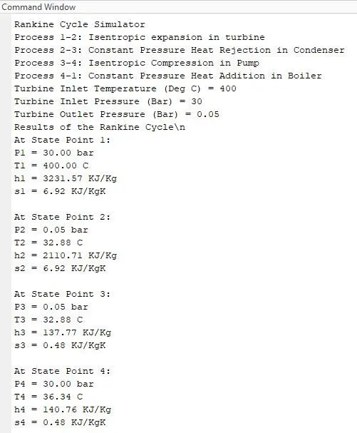
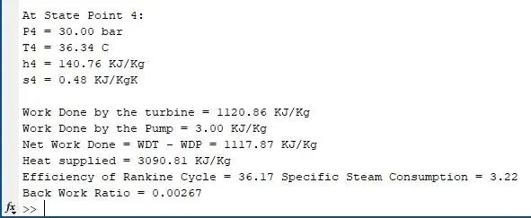
In the results section, we first display all the parameters at various state points using a floating format specifier corrected to 2 decimal places. Then we compute the various performance parameters like work, efficiency, heat supplied etc. and are displayed accordingly as shown in the output command window.
OUTPUTS:
GRAPHS: