Project 2 - Rankine cycle Simulator

* OBJECTIVE: The main objective of this challenge is to create a rankine cycle simulator and calculate the state points based on the user inputs and plot the corresponding T-s and h-s plots.

* RANKINE CYCLE:

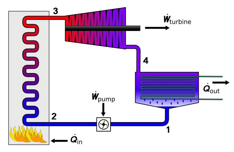
The Rankine cycle is a model used to predict the performance of steam turbine systems. It was also used to study the performance of reciprocating steam engines. The Rankine cycle is an idealized thermodynamic cycle of a heat engine that converts heat into mechanical work while undergoing phase change. It is an idealized cycle in which friction losses in each of the four components are neglected. The heat is supplied externally to a closed loop, which usually uses water as the working fluid.

* Processes in Rankine Cycle:
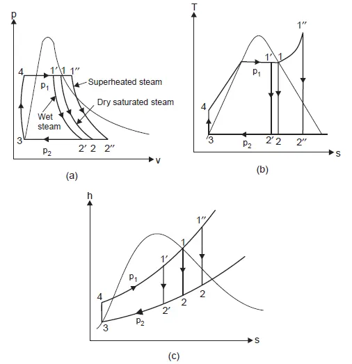
There are four processes in the Rankine cycle. These states are identified by numbers (in brown) in the above T–s diagram. Process 1-2 : Reversible adiabatic expansion in the turbine.
Process 2-3 : Constant-pressure transfer of heat in the condenser.
Process 3-4 : Reversible adiabatic pumping process in the feed pump.
Process 4-1 : Constant-pressure transfer of heat in the boiler.

Applying steady flow energy equation (S.F.E.E.) to boiler, turbine, condenser and pump :
(i) For boiler (as control volume)
f4 + Q1 = h1
∴ Q1 = h1 – hf4
(ii) For turbine (as control volume)
h1 = WT + h2, where WT = turbine work
WT = h1 – h2
(iii) For condenser
h2 = Q2 + hf3
∴ Q2 = h2 – hf3
(iv) For the feed pump
hf3 + WP = hf4 , where, WP = Pump work
∴ WP = hf4– hf3 = v3 (p1 – p2)
Efficiency of Rankine cycle is given by
η =W/Qnet1=WT-WP/Q1

* INPUTS:

Pressure at state point 1(turbine inlet), [p1] = 30, bars
Temperature at state point 1(turbine inlet), [T1] = 400, degree celsius
Pressure at state point 2(turbine outlet), [p2] = 0.05, bars

% Rankine Cycle Simulator
clear all
close all
clc

% Printing Introduction
fprintf('RANKINE CYCLE SIMULATOR \n')
fprintf('\n1-2 is isentropic expansion in the Turbine \n')
fprintf('2-3 is Constant Pressure Heat Rejection by the Condenser \n')
fprintf('3-4 is isentropic Compression in pump \n')
fprintf('4-1 is Constant Pressure Heat Addition by the Boiler \n')

% User Inputs
P1 = input('\nEnter the Pressure at the Turbine Inlet (in bar): ');
T1 = input('Enter the Temprature at the Turbine Inlet (in Degree Celcius): ');
P2 = input('Enter the Pressure at the Turbine Outlet (in bar): ');

% State point 1
H1 = XSteam('h_pt',P1,T1);  %Enthalpy
S1 = XSteam('s_pt',P1,T1);  %Entropy
Hf1 = XSteam('hL_p',P1);    %Enthalpy of saturated liquid
Hg1 = XSteam('hV_p',P1);    %Enthaply of saturated vapour
Ts1 = XSteam('Tsat_p',P1);  %Saturation Temprature
Sf1 = XSteam('sL_p',P1);    %Entropy of saturated liquid
Sg1 = XSteam('sV_p',P1);    %Entropy of saturated vapour

% State point 2
S2 = S1;
Sf2 = XSteam('sL_p',P2);
Sg2 = XSteam('sV_p',P2);
x = (S2-Sf2)/(Sg2-Sf2);     % Dryness fraction
Hf2 = XSteam('hL_p',P2);
Hg2 = XSteam('hV_p',P2);
H2 = Hf2 + x*(Hg2-Hf2);
T2 = XSteam('T_ph',P2,H2);
Ts2 = XSteam('Tsat_p',P2);   

% State point 3
H3 = Hf2;
S3 = Sf2;
T3 = T2;
P3 = P2;

% State point 4
P4 = P1;
S4 = S3;
H4 = XSteam('h_ps',P4,S4);
T4 = XSteam('T_ps',P4,S4);

t = linspace(0,374,500);    % temp space for plotting saturation cutves

%Plot T-S Diagram
figure(1)
hold on
% Plot Saturation Curve
for i = 1 : length(t)
   plot(XSteam('sL_T',t(i)),t(i),'.','color','b')
   plot(XSteam('sV_T',t(i)),t(i),'.','color','b')
end
% Plot Cycle
plot([S1 S2],[T1 T2],'linewidth',2,'color','r')
if x>1
    T3 = Ts2;
    plot([S2 Sg2 S3 S4],[T2 Ts2 T3 T4],'linewidth',2,'color','r')
    T2 = Ts2;
else
    plot([S2 S3 S4],[T2 T3 T4],'linewidth',2,'color','r')
end
l = linspace(T1,T2,1000);
for i = 1 : length(l)
    plot(XSteam('s_pT',P1,l(i)),l(i),'.','color','r')
end
plot([Sf1 Sg1],[Ts1 Ts1],'linewidth',2,'color','r')
xlabel('Entropy[KJ/Kg-K]')
ylabel('Temprature[degree celsius]')
title('T-S Diagram')

% Plot H-S Diagram
figure(2)
hold on
% Plot Saturation Curve
for i = 1 : length(t)
    plot(XSteam('sL_T',t(i)),XSteam('hL_T',t(i)),'.','color','b')
    plot(XSteam('sV_T',t(i)),XSteam('hV_T',t(i)),'.','color','b')
end
% Plot Cycle
plot([S1 S2 S3 S4 S1],[H1 H2 H3 H4 H1],'linewidth',2,'color','r')
xlabel('Entropy[KJ/Kg-K]')
ylabel('Enthalpy[KJ/Kg]')
title('H-S Diagram')

% calculations

% Turbine Work
Wt = H1-H2;

% Pump Work
Wp = H4-H3;

% Heat Addition
Qin = H1-H4;

% Heat Rejection
Qout = H2-H3;

% Net Work
Wnet = Wt-Wp;

% Efficiency
Ntherm = (Wnet/Qin)*100;

% Specific steam consumption
SSC = 3600/Wnet;

% Back Work Ratio
BWR = Wp/Wt;

% Print Results
fprintf('\n\nResults\n')
fprintf('At State Point 1:\n')
fprintf('P1 is : %.2f bar\n',P1)
fprintf('T1 is : %.2f Deg Celcius\n',T1)
fprintf('H1 is : %.2f KJ/Kg\n',H1)
fprintf('S1 is : %.2f KJ/Kg-K\n',S1)

fprintf('\nAt State Point 2:\n')
fprintf('P2 is : %.2f bar\n',P2)
fprintf('T2 is : %.2f Deg Celcius\n',T2)
fprintf('H2 is : %.2f KJ/Kg\n',H2)
fprintf('S2 is : %.2f KJ/Kg-K\n',S2)

fprintf('\nAt State Point 3:\n')
fprintf('P3 is : %.2f bar\n',P3)
fprintf('T3 is : %.2f Deg Celcius\n',T3)
fprintf('H3 is : %.2f KJ/Kg\n',H3)
fprintf('S3 is : %.2f KJ/Kg-K\n',S3)

fprintf('\nAt State Point 4:\n')
fprintf('P4 is : %.2f bar\n',P4)
fprintf('T4 is : %.2f Deg Celcius\n',T4)
fprintf('H4 is : %.2f KJ/Kg\n',H4)
fprintf('S4 is : %.2f KJ/Kg-K\n',S4)

fprintf('\nWt is : %.2f KJ/Kg\n',Wt)
fprintf('Wp is : %.2f KJ/Kg\n',Wp)
fprintf('Wnet is : %.2f KJ/Kg\n',Wnet)
fprintf('Thermal Efficiency is : %.2f percent\n',Ntherm)
fprintf('S.S.C. is : %.2f Kg/KWh\n',SSC) 
fprintf('Back Work Ratio is : %.3f \n',BWR)

* Step- wise exlination of code:

1. Xsteam data is used to extract steam and water properties of enthalpy and entropy at specific pressure and temperature.
2. The program requires Pressure [p1](in bar) at state point 1 (turbine inlet), Temperature[T1] at the same state point (degree Celsius) and Pressure[p2] at the turbine outlet (in bars)
3. With the help of these inputs, the program calculates all the state points of the Rankine cycle with Xsteam data.
4. The Enthalpy can be calculated as h1 = Xsteam ('h_pT', p1, T1); (Returns the enthalpy of water at given pressure in bars and Temperature in degree Celsius)
5. 5.Thermodynamic relations are used further to find state points. The below relations are used to find the state points at state point 1

H1 = XSteam('h_pt',P1,T1)

S1 = XSteam('s_pt',P1,T1)

Hf1 = XSteam('hL_p',P1)

Hg1 = XSteam('hV_p',P1)

Ts1 = XSteam('Tsat_p',P1)

Sf1 = XSteam('sL_p',P1)

Sg1 = XSteam('sV_p',P1)

6. Sf and sg, hf and hg,

where f and g are saturated liquid and saturated vapour respectively.

7. The net-work, work done by turbine, work done to run the pump, heat in, heat out, Efficiency, Specific steam consumption (S.S.C) and back work ratio of the Rankine cycle are calculated by using standard relations

- For boiler (as control volume)
f4 + Q1 = h1
∴ Q1 = h1 – hf4
- For turbine (as control volume)
h1 = WT + h2, where WT = turbine work
∴ WT = h1 – h2
- For condenser
h2 = Q2 + hf3
∴ Q2 = h2 – hf3
- For the feed pump
hf3 + WP = hf4,

where, WP = Pump work
∴ WP = hf4– hf3 = v3 (p1 – p2)
- Efficiency of Rankine cycle is given by
η =W/Qnet1=WT-WP/Q1

- Specific steam consumption (S.S.C)

SSC = 3600/Wnet;

- Back work ratio (BWR)

BWR = Wp/Wt;

8. Temperature (T), Entropy (s) and Enthalpy (h) are extracted at vapour and liquid line for plotting purpose, after 4th point for the variation you observe in the plot.
9. Plot of T-s and h-s is created from all the points calculated the program.
10. The plot changes according to the user inputs (p1, T1, p2).
11. Results are displayed in the command window.

* REFERENCES:
1. https://www.slideshare.net/akashdjkid/rankine-cycle-12868084

2.https://en.wikipedia.org/wiki/Rankine_cycle

3. https://unacademy.com/lesson/derivation-of-rankine-cycle-efficiency/6N3PYQ4O

4. http://www.nuclear-power.net/nuclear-engineering/thermodynamics/thermodynamic-cycles/rankine-cycle-steam-turbine-cycle/theory-of-rankine-cycle-equations-and-calculation/