Project 1

OBJECTIVE:

• The main objective is to develop a forward model energy-based fuel consumption of a conventional vehicle, in Simulink to analize the vehile performance and writing a program to plot different parameter in matlab.

1. Build the Simulink model (Engine and vehicle Dynamics block) by using different block in simulink library.
2. Writing scripts in Matlab to load the variables, those are required to run the simulink model and plotting the different paramenters.
3. Tabulate the fuel econony numbers (kmpl) for UDDS and HWFET cycles.
4. Plot the time trace for engine, Transmission input, Transmission output and wheel speed on one plot.
5. Plot engine torque, engine power, fuel rate and fuel consumption using subplots.
6. Plot accelerator and break pedal, gear command, vehicle desired and actual speed, vehicle distance using sub plots.
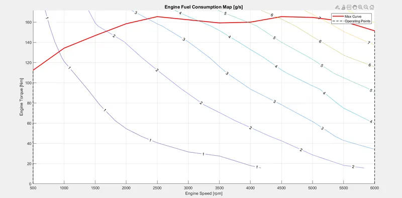
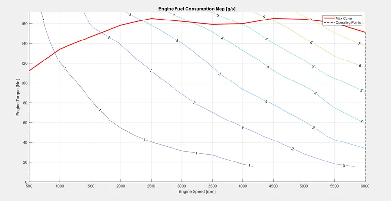
7. Plot engine operating points on the engine fuel map.
8. Generate the plots for both drive cycles.
9. Study of conventional vehicle simulink model and creates graphs.

Conventional vehicle:

Conventional vehicles use an internal combustion engine fuelled by gasoline or diesel, to power the wheels. In this the heat engine uses the principle of heat release through combustion of fuel with an oxidizer in a combustion chamber to create expanding gases which pushes against a piston creating force and torque output

In the Internal combustion (IC) engines, chemical energy of fuel is converted in to the heat energy to produce useful mechanical work. Mostly uses fossil fuels like petroleum (petrol and diesel).

The most common type of engines are 4 stroke reciprocating engines. The internal combustion or conventional vehicle is operated based on the Ideal thermodynamic cycles such Otto cycle, Diesel cycle, over expanded cycle and etc.

Energy and Performance of the vehicle:

In this system, the power is supplied from the powertrain to wheels to operate the vehicles. In other words, the power coming from the powertrain dictates the power demand on the wheels (as per performance viz, acceleration, speed and etc. is determined by it).

In this type of vehicles, the powertrain consists of an engine connected to the wheels through the transmission and differential, therefore the power/energy is transmitted to the wheels.

Conventional Powertrain Efficiency:

The engine generates the power by converting the chemical energy of fuel into heat energy and then useful mechanical energy by the processes of combustion. This process of energy of energy conversion has an efficiency and the energy input is in the form of fuel combustion.

Instantaneous fuel combustion is given below,

`mf = (Pe)/(etae.etat.QLHV)`

Here,

`mf` = mass flow rate [kg]

`Pe` = power of engine

`pt` = power transmission

`etat` = efficiency of transmission

`etae` = efficiency of engine

`QLHV` = lower heating value/the calorific value

The internal combustion engines consume the power even if the vehicle is in idle position, to overcome the engine drag loss and keep it spinning, this is the idling fuel consumption and know as idling process. The fuel consumption is not only depending on the power requirement at the wheels, the engine consume the power to run the different components of the vehicle.

System Dynamics:

The system dynamics deals with the modeling of multi domain systems, through the use of a unified approach based on an ordinary differential and algebraic equation describing the static and dynamic effects.

Generally, each system has three variables those are Efforts, Flow and power.

1. Efforts: It is generalized force variable [Ex. Torque, force, voltage, heating value and etc.]
2. Flow: It is the generalized flow/velocity variables [Ex. Velocity, mass flow rate and etc.]
3. Power: It is the product of the effort and flow variable. It is interchangeable between the energy domains.

Energy based models – Element models:

To model the internal physical properties of the element and the losses, there are two kinds of approaches, those are Map based models and Analytical models.

1. Map based models:

Elements are modeled using maps, which characterize the relationship between the input & output and output & losses etc.

2. Analytical models:

Elements are modeled using physical equations, that represent the internal dynamics.

Different types of efficiencies:

• Mechanical efficiency:

It is the ratio of brake power (B.P) to the indicated power (I.P).

• Overall efficiency:

It is the ratio of work obtained at the crankshaft in a given time to the energy supplied by the fuel during same time.

• Indicated thermal efficiency:

It is the ratio of the heat equivalent to one kW-hr to the heat in the fuel per I.P hr.

• Brake thermal efficiency:

It is the ratio of the heat equivalent to one kW-hr to the heat in the fuel per B.P hr.

• Volumetric efficiency:

It is the ratio of the actual volume of charge admitted during the suction stroke at N.T.P to the swept volume of the position.

Matlab program:

%%%%%%%%%%%%%%%%%%%%%%%%%%%%%%%%%%%%%%%%%%%%%%%%%%%%%%%%%%%%%%%%%%%%%
clc
%% Skill-Lync -> Hybrid Drives Development
% Project 1 - Conventional Vehicle Model
% By - Ullekh Gambhira 

% Description:

%% Initialization File
% Initialization file for loading the variables for the Conventional vehicle simulation model

%% Vehicle Parameters
M = 1500;       % Vehicle weight [kg]
Cr = 0.015;     % Rolling resistance coefficient
Rw = 0.35;      % Rolling radius [m]
Cd = 0.33;      % Drag coefficient
Af = 2;         % Frontal area [m2]
rhoa = 1.225;   % Air density [kg/m3]
Vwind = 0;      % Wind velocity [kmph]
g = 9.81;       % Gravitational acceleration [m/s2]
theta = 0;      % Slope [deg]
myu_road_tire = 1; % Coefficient of friction between tire - road interface

%% Powertrain Parameters 
FDR = 3.73;                         % Final Drive Ratio / Diff Ratio
DiffEff = 0.99;                     % Differential efficiency (assumed independent of operating conditions)

NumGear = 4;                        % Number of gears in transmission
TransGear = [1:NumGear];            % Transmission Gears
TransRatio = [3.06, 1.62, 1, 0.7];  % Corresponding Transmission ratios
TransEff = 0.90;                    % Transmission efficiency (assumed independent of operating conditions)

TC_SR = [0, .5, .6, .7, .8, .87, .92, .94, .96, .97, 1];   % Torque Converter Speed Ratio (Matlab default) -> TurbSpd/PumpSpd  
TC_TR = [2.232, 1.5462, 1.4058, 1.2746, 1.1528, 1.0732, 1.0192, 1, 1, 1, 1];   % Torque Converter Torque Ratio (Matlab default) -> TurbTrq/PumpTrq
TC_Cf = 1e-4 * [.72558, .66322, .63463, .59042, .51331, .4144, .29287, .22444, .12186, .04386, 0]; % Torque Converter Capacity Factor (Matlab default) -> PumpTrq/PumpSpd^2 [Nm/rpm^2]

load Vehicle_Data/Engine_data_1_9L_Saturn_95kW
load Vehicle_Data/Trans_Shift_map

%% Driver Parameters
Kp = 10;                    % P gain for driver PI model
Ki = 1;                     % I gain for driver PI model
Drive_Cycle_Select = 1;     % Drive cycle selection

% Drive cycle values in m/s

if Drive_Cycle_Select == 1
    load DriveCycles/UDDS;
    
elseif Drive_Cycle_Select == 2
    load DriveCycles/HWFET;
    
elseif Drive_Cycle_Select == 3
    load DriveCycles/FTP;
    
elseif Drive_Cycle_Select == 4
    load DriveCycles/US06;
    
elseif Drive_Cycle_Select == 5
    load DriveCycles/NEDC;
    
elseif Drive_Cycle_Select == 6
    load DriveCycles/WLTP;
 
end

time_end = cyc_time(end);
vel_end = cyc_vel(end);

• The above MATLAB program is used to load the required variables to run the Simulink model and for post processing.
• The drive cycle selection also done here, before run the Simulink vehicle model run this initialization script.
• The program developed has the capability to simulate the vehicle on different rive cycles like UDDS, HWFET, FTP, NEDC and etc.

The Simulink model:

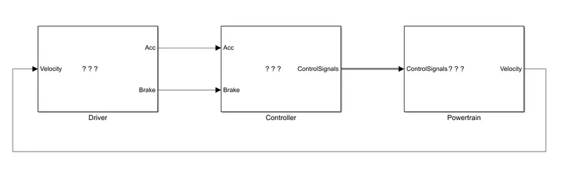
In this project a typical midsize car with 1.9L engine and a 4-speed automatic transmission is considered. Data taken from ADVISOR data base developed by NREL, USA transmission shift map and controller is taken from MATLAB/Simulink example database.

>> Vehicle Model:

>> Driver Model: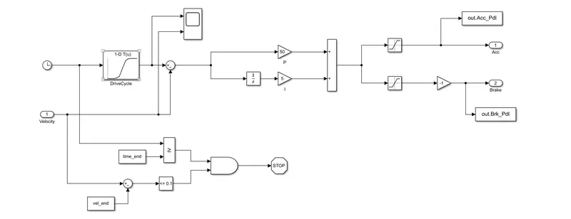

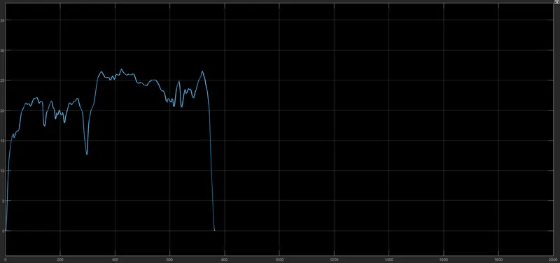
The driver block is a basic PI controller that generates accelerator and brake pedal outputs to match the desired & actual vehicle speeds. The feedback loop is connected to this driver block form the powertrain block. The feedback loop is used to optimize the vehicle speed and other perameters.

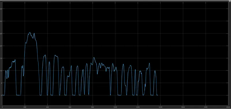
Scope block graphs for Driver Model:

For UDDS drive cycel:

For HWFET drive cycle:

>> Controller Model:

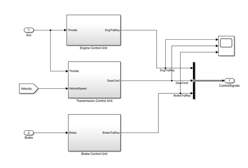
The controller block is main component of the vehicle model, it has 3 electronic control units Engine control unit, Transmission control unit and Brake control unit. All 3 electronic control units are connected to single scope, to visualize and understand the performance of the controller model.

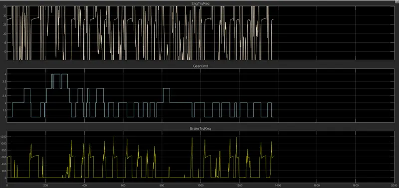
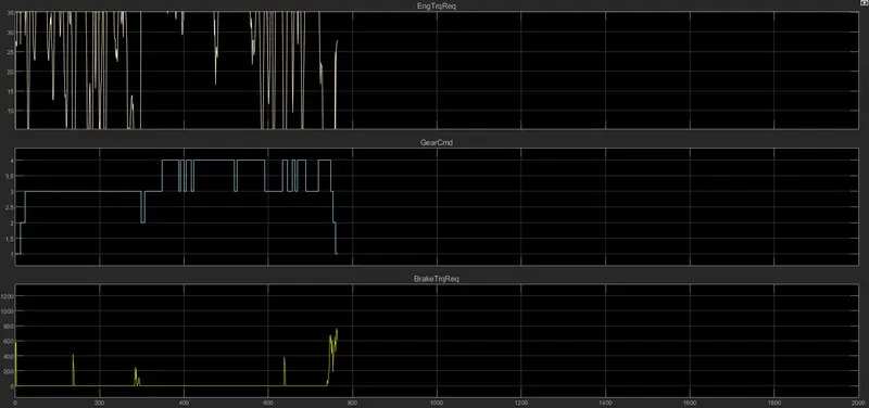
Scope block graphs for Controller Model:

For UDDS drive cycle:

For HWFET deive cycle:

** Engine Control Unit Model:

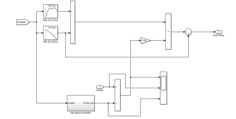
In this engine control unit, used 2 look up tables to input the maximum and minimum torque values. The input for the look up tables are fed through the EngSpd goto block, the engine speed also given to ideal control speed to integrate from this to meet the output of the engine required torque. The engine control unit has a subsystem called Ideal speed controller.

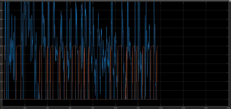
Scope block graphs for Engine Control Unit Model:

for UDDS drive cycle:

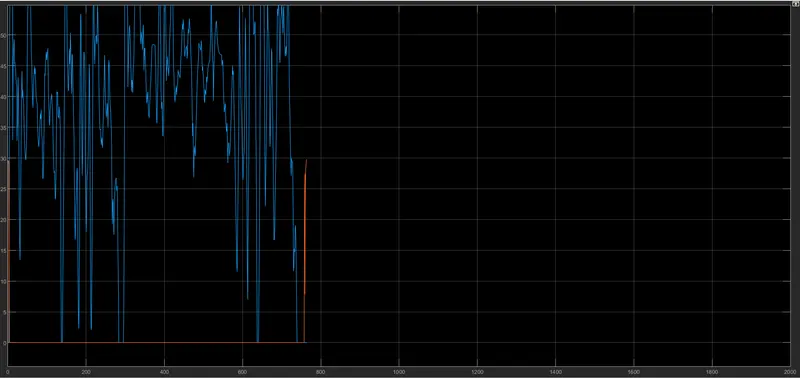
for HWFET drive cycle:

** Transmission Control Unit Model:

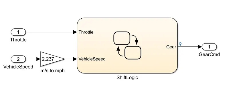
The Transmission control unit fed with the 2 inputs (acceleration and the velocity). In the transmission control unit the shift logic is used for controlling the gears as in the ascending and descending order wrt time, speed and distance.

** Brake Control Unit Model:

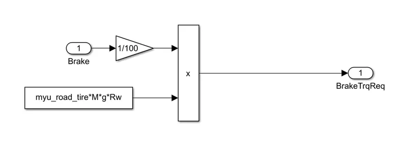
The brake control unit fed with an input of Brake data. In this brake control unit, the brake torque is calculated.

>> Powertrain Model:

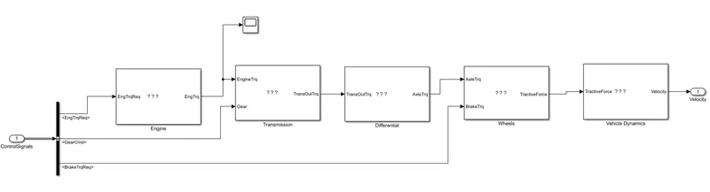
The powertrain is the model, that encompasses every component that converts the power from the engine into mechanical movement. This powertrain model has Engine, Transmission, Differential, Wheels, Vehicle dynamics blocks. From this powertrain block a feedback loop is connected to the driver block to check the different parameters performance and to optimize the vehicle movement. the scope block is connected after the engine block to check the output from the engine, the output from the engine is connected to the transmission block.

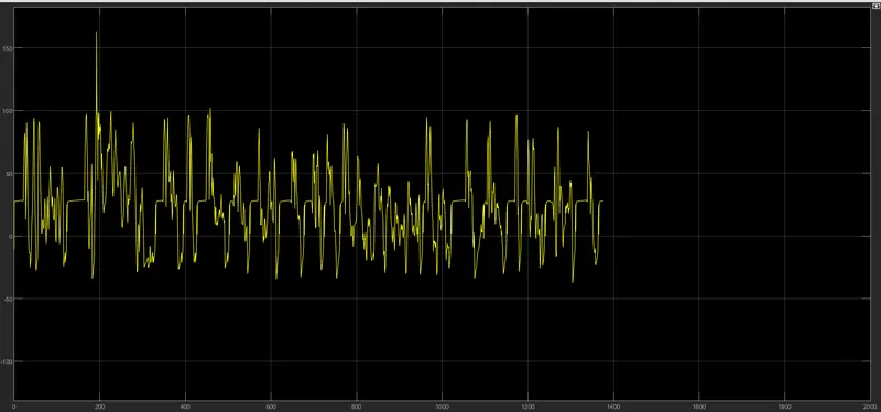
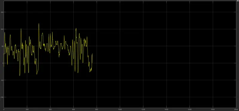
the blow scope block is connceted after the engine block in the Powertrain model,

for UDDS fdrive cycle:

for HWFET drive cycle:

** Engine Model:

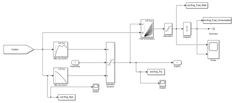
In this engine block, the map-based models are used to model the fuel consumption of the engine. It is based on maximum torque and minimum torque of the controller. In this model I have used the look up tables to input the toque data, and the min torque, max torque and the EngTrqReq block is connected to the dynamic saturation input block and the output from the dynamic saturation block is connected to EngTrq block (the output of the engine block) and to 2D look up table (2D look up table get fed the inputs from the dynamic saturation block and the min torque data). The output from the 2d look up table is connected to the saturation block to get the engine fuel rate, and then connected to integrator block to get the fuel consumption.

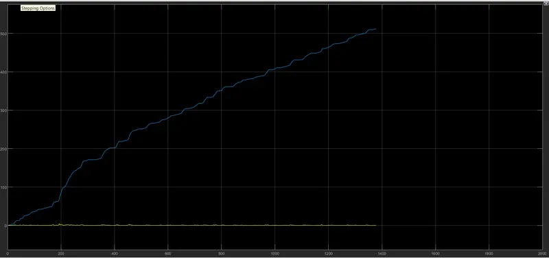
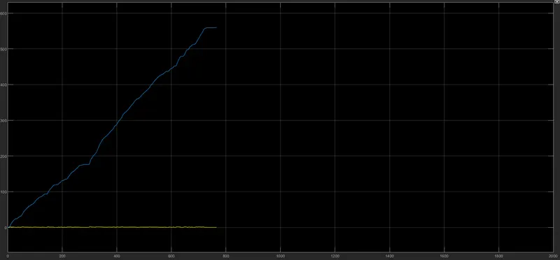
Scope blocks graphs for Engine Model:

For UDDS drive cycle:

For HWFET drive cycle:

** Transmission Model:

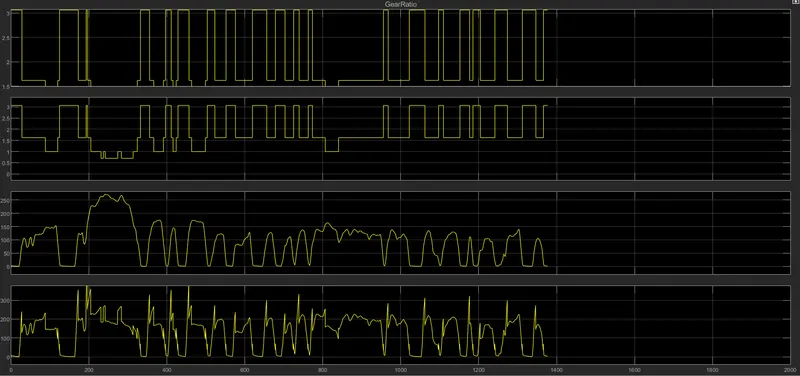
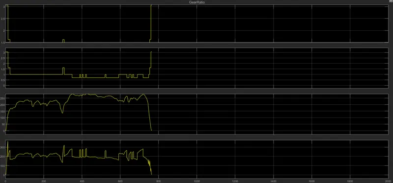
The transmission block takes the input from the engine block (engine torque), the gear selector from controller for transmission of gear ratio, the gear ration is multiplied by the transmission input torque. The output from the torque converter block is connected to the product block to get the transmission out torque.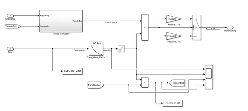

*Torque Converter Model: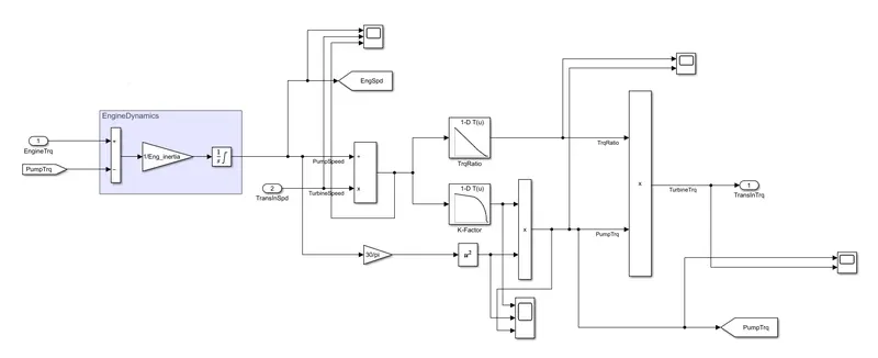

Scope block graphs for Transmission Model:

For UDDS drive cycle:

For HWFET drive cycle:

** Differential Model:

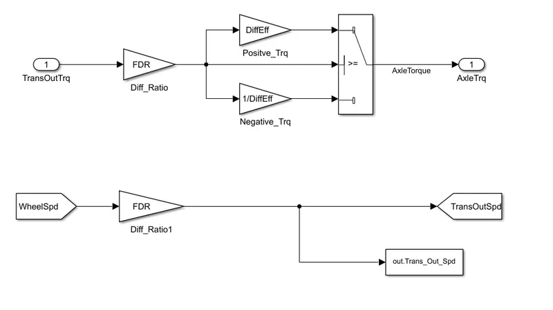
In this differential model, the inputs are fed with the output block of the transmission model (TransOutTrq), this input is multiplied with the differential ratio, the differential ratio get multiplied with output and input torque to get the axle torque. The differential ratio and the transmission torque are greater than the axle torque.

** Wheels Model:

For this wheel model the input is axle torque and brake torque, the axle torque is the differential model output and the brake torque is from the brake control unit. These inputs are subtracted and the output is get multiplied with rolling radius to get the tractive force. The rolling radius and velocity are multiplied to get the wheel speed.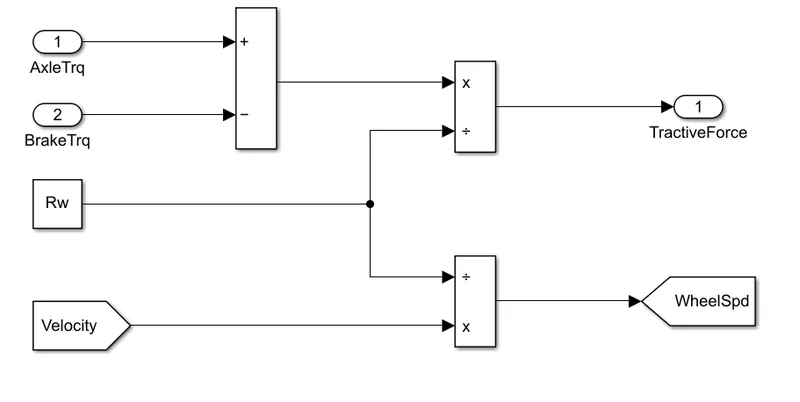

** Vehicle Dynamics Model:

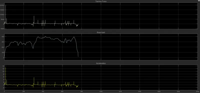
The vehicle dynamics model takes the tractive force as an input. The vehicle dynamics dictates the vehicle speed based on the tractive force and road load. The below equation is used for calculating the road load. The equation is,

`Meq (dVveh)/dt = (etatlambda)/(Rw) . Tm - (1/2.rhoa.Af.Cd(Vveh + Vw)^2 + Cr.Mgcostheta + Mgsintheta)`

where,

`rhoa` = Air density `[(kg)/m^3]`
`Af` = Frontal area `[m^2]`
`Cd` = Drag coefficient
`Vveh` = Velocity of vehicle `[m/s]`
`Vw` = Velocity of wind (or) Head wind `[m/s]`
`Cr` = Rolling resistance coefficient
`M` = Mass `[kg]`
`g` = Gravitational force

`theta` = Angel (or) grade

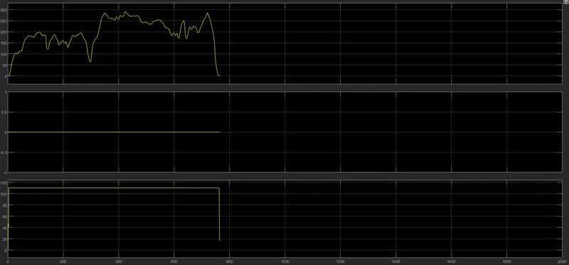
The output from the road load is connected to an add block, another input for add block is tractive force. The mass and sum of tractive force & road load is connected to the divide block to get acceleration, the divide block is connected to integrator block to get vehicle speed. The integrator output (velocity) is connected to one more integrator block to know the vehicle distance. The output velocity is connected to the driver block as an input.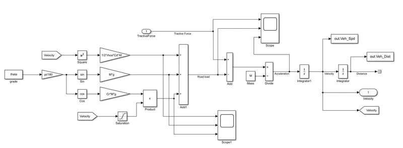

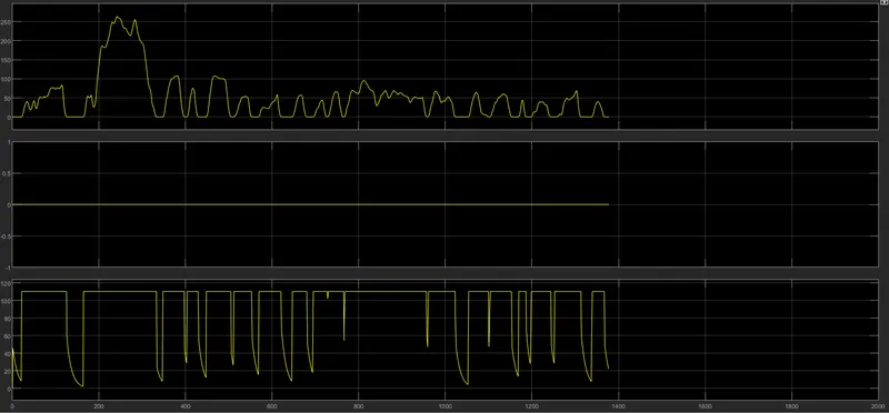
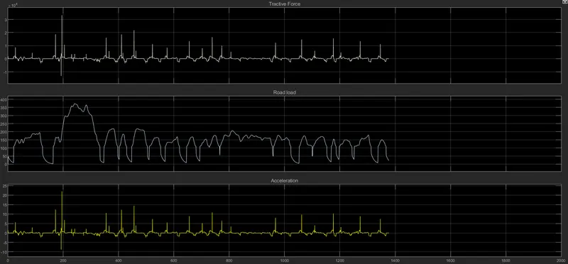
Scope block graphs for Vehicle Dynamics Model:

For UDDS drive cycle:

Scope-1

Scope-2

For HWFET drive cycle:

Scope-1

Scope-2

Once the Simulink vehicle model simulation was done, some data will be sent to the MATLAB workspace with the help of 'To workspace' block. The data from the Simulink model is helps to plot the different parameters of the conventional vehicle in MATLAB.

The below modified program is used to plot the following parameters for both UDDS and HWFET drive cycles,

1. Trans input, Trans output and Wheel speed.
2. Engine Torque, Engine Power, Engine Fuel Rate and Engine Fuel Consumption.
3. Fuel Economy vs Fuel Consumption.
4. Acceleration, Brake pedal and gear command with respect to time.
5. Gear command with respect to vehicle speed and distance.
6. Engine Fuel Consumption map [g/s].

%%%%%%%%%%%%%%%%%%%%%%%%%%%%%%%%%%%%%%%%%%%%%%%%%%%%%%%%%%%%%%%%%%%%%
clc
close all
%% Skill-Lync -> Hybrid Drives Development
% Project 1 - Conventional Vehicle Model 

% Description:
% The following file is to used with the Initialization file and Simulink
% results for post-processing of the data.
% The file is incomplete, has some examples of how the data is imported
% into a readable format, data analysis and plotting examples.
% Based on the project task, use commands in a similar format as given
% below, to analyse the data and generate required plots.
% You can change variable names if desired

%% Post-Processing File
%  File for post-processing the Conventional vehicle simulation model data

%% Renaming variables
Time = out.tout;
Acc_Pdl = out.Acc_Pdl;                          % Accelerator pedal [%]
Brk_Pdl = out.Brk_Pdl;                          % Brake pedal [%]
Gear_Cmd = out.Gear_Cmd;                        % Transmission gear
Trans_In_Spd = out.Trans_In_Spd*30/pi;          % Transmission input speed [rpm]
Trans_Out_Spd = out.Trans_Out_Spd*30/pi;        % Transmission output speed [rpm]
Eng_Trq = out.Eng_Trq;                          % Engine brake torque [Nm]
Eng_Spd = out.Eng_Spd*30/pi;                    % Engine speed [rpm]
Eng_Fuel_Consump = out.Eng_Fuel_Consumption;    % Engine fuel consumption [g]
Veh_Dist = out.Veh_Dist/1000;                   % Distance traveled by vehicle [km]
Veh_Spd = out.Veh_Spd*18/5;                     % Vehicle speed [kmph]
Wheel_Speed = out.wh_speed;                     % Wheel speed [kmph]
Eng_Fuel_Rate = out.Eng_Fuel_Rate;              % Engine fuel rate [%]


%% Data Analysis
Eng_Pwr = Eng_Spd*pi/30*Eng_Trq/1000;                            % Engine brake power [kW]
rho_petrol = 0.7197;                                             % Density of petrol [kg/L]
kmpl = Veh_Dist(end)/(Eng_Fuel_Consump(end)/1000/rho_petrol);    % Fuel economy [kmpl] 


%% Plotting Vehicle characteristics time trace transmission IN/OUT and Wheel speed

figure(1)
hold on
grid on
plot(Time, Trans_In_Spd, 'linewidth', 1,'color', 'k')
plot(Time, Trans_Out_Spd, 'linewidth', 1, 'color', 'r')
plot(Time, Wheel_Speed, 'b')
xlabel('Time [s]')
ylabel('Speed [rpm]')
xlim([0, Time(end)]);
ylim([0,6000]);
legend('Trans Input', 'Trans Output', 'Wheel Speed')

%% Plotting Vehicle characteristics time trace Engine speed, Engine Torque, Engine Power, Engine fuel rate and Engine fuel consumption
%Data conversion from Double Time series

Eng_spd = Eng_Spd.Data(:,1);                       % Engine speed
Eng_trq = Eng_Trq.Data(:,1);                       % Engine torque
Eng_pwr = Eng_Pwr.Data(:,1);                       % Engine power
Eng_fuel_rate = Eng_Fuel_Rate.Data(:,1);           % Engine fuel rate
Eng_fuel_consumption = Eng_Fuel_Consump.Data(:,1); % Engine fuel consumption
Veh_dist = Veh_Dist.Data(:,1);                     % Vehicle distance
Veh_spd = Veh_Spd.Data(:,1);                       % Vehicle speed

% Plotting Engine speed, Engine Torque, Engine Power, Engine fuel rate, Engine fuel consumption wrt time 

figure(2)
subplot(2,2,1)
plot(Time, Eng_trq, 'linewidth', 1, 'color', 'k')
xlabel('Time [s]')
ylabel('Toque [Nm]')
legend('Engine Torque')

grid on
subplot(2,2,2)
plot(Time, Eng_pwr, 'linewidth', 1, 'color', 'b')
xlabel('Time [s]')
ylabel('Power [kW]')
legend('Engine Power')

grid on
subplot(2,2,3)
plot(Time, Eng_fuel_rate, 'linewidth', 1, 'color', 'r')
xlabel('Time [s]')
ylabel('Fuel Rate [%]')
legend('Engine Fuel Rate')

grid on
subplot(2,2,4)
plot(Time, Eng_fuel_consumption, 'linewidth', 1, 'color', 'g')
xlabel('Time [s]')
ylabel('Fuel Consumption')
legend('Engine Fuel Consumption')
grid on

% Plotting Fuel Economy vs Engine Fuel Consumption

figure(3)
plot(Eng_fuel_consumption, Eng_fuel_rate, 'color', 'r')
xlabel('Fuel Consumtion')
ylabel('Fuel Rate [%]')
title('Fuel Economy vs Fuel Consumption')
grid on

%% Plotting Acceleration pedal, Brake pedal and gear command wrt time
figure(4)
subplot(2,1,1)
hold on
plot(Time, Acc_Pdl, 'linewidth', 1, 'color', 'k')
plot(Time, Brk_Pdl, 'linewidth', 1, 'color', 'r')
xlabel('Time [s]')
ylabel('Pedal [%]')
xlim([0, Time(end)]);
grid on
legend('Accel', 'Brake')
title('Acceleration &Brake pedal wrt Time')

subplot(2,1,2)
plot(Time, Gear_Cmd, 'linewidth', 1, 'color', 'k')
xlim([0, Time(end)]);
xlabel('Time [s]')
ylabel('Gear')
grid on
title('Gear command wrt Time')

% Plotting gear command vehicle desired with actual speed

figure(5)
subplot(2,1,1)
plot(Veh_spd, Gear_Cmd, 'linewidth', 1, 'color', 'k')
xlabel('Speed [rpm]')
ylabel('Gear')
grid on
title('gear Command wrt Vehicle Speed')

subplot(2,1,2)
plot(Veh_dist, Gear_Cmd, 'linewidth', 1, 'color', 'r')
xlabel('Distance [kmpl]')
ylabel('Gear')
grid on
title('Gear command wrt distance')


%% Plotting engine operating points on engine fuel map

figure('Name','Engine Operating Points');
hold on
grid on
title('Engine Operating Points','fontsize',12);
p1=plot(Eng_map_spd*30/pi,Eng_max_trq,'linewidth',2,'color','r');
p2=line([Eng_map_spd(end)*30/pi Eng_map_spd(end)*30/pi],[0 Eng_max_trq(end)]);
set(p2,'linewidth',1,'linestyle','--','color','k');
p3=line([Eng_map_spd(1)*30/pi Eng_map_spd(1)*30/pi],[0 Eng_max_trq(1)]);
set(p3,'linewidth',1,'linestyle','--','color','k');
[c,h] = contour(Eng_map_spd'*30/pi,Eng_map_trq,Eng_fuel_map');
clabel(c,h);
xlabel('Engine Speed [rpm]');
ylabel('Engine Torque [Nm]');
title('Engine Fuel Consumption Map [g/s]');
legend([p1 p3],{'Max Curve','Operating Points'});
axis([Eng_map_spd(1)*30/pi Eng_map_spd(end)*30/pi 0 Eng_map_trq(end)]);

Plots for UDDS and HWFET Drive Cycles:

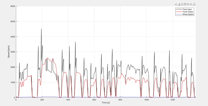
1. Plotting the Vehicle characteristics time trace, Transmission IN/OUT and Wheel speed:

For UDDS drive cycle:

For HWFET drive cycle:

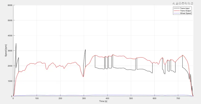
In these above graphs we can observe and understood from where thw transmission input speed starts and where the transmission output speed will stops and we can able to obser the wheel speed also.

2. Plotting the vehicle characteristics Time trace to Engine Torque, Engine Power, Engine Fuel Rate and Engine Fuel Consumption:

For UDDS drive cycle:

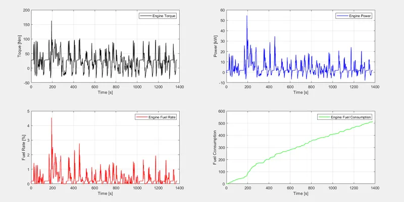
For HWFET drive cycle:

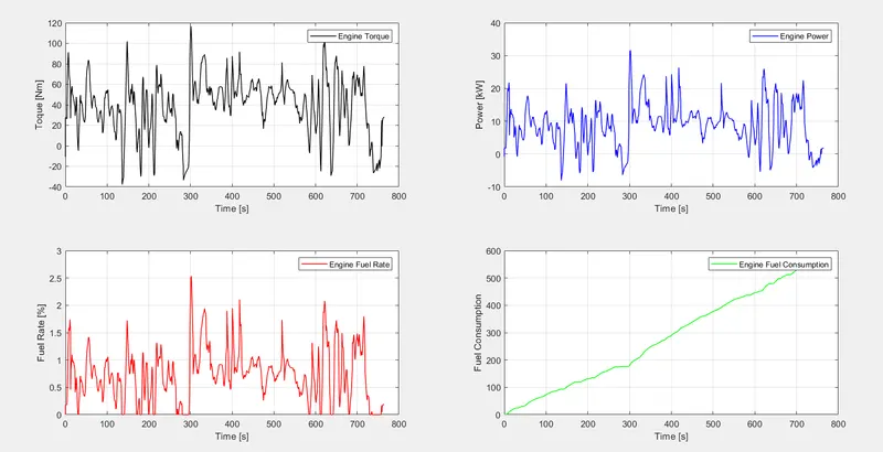
in those above graphs we can observe,

- With respect to time the engine torque will be high at some points and low at some points.

- With respect to time the engine power will be high at some points and low at some points.

- With respect to time the engine fuel rate will be increasing at some points and decresing at some points.

- With respect to time the engine fuel consumption will be increasing gradually.

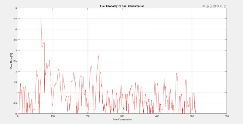
3. Plotting the Fuel Economy vs Fuel Consumption:

For UDDS drive cycle:

For HWFET drive cycle:

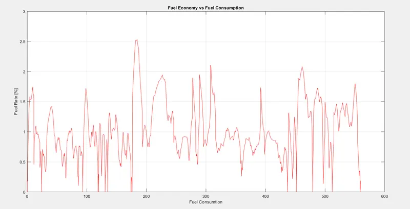
In those graphs we can observe the abrput increase and decrease of fuel rate with respect to the fuel consumption.

4. Plotting the Accelerator pedal, Break pedal and Gear command with respect to time:

For UDDS drive cycle:

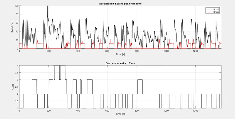
For HWFET drive cycle:

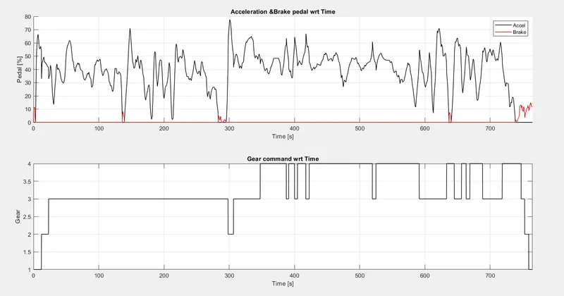
In those graphs we can observe that, the brake of vehicle and the acceleration of vehicle is more so the brake torque is minimum required, and the gear shifting is required with respect to time.

5. Plotting Gear command with respect to vehicle speed and distance:

For UDDS drive cycle:

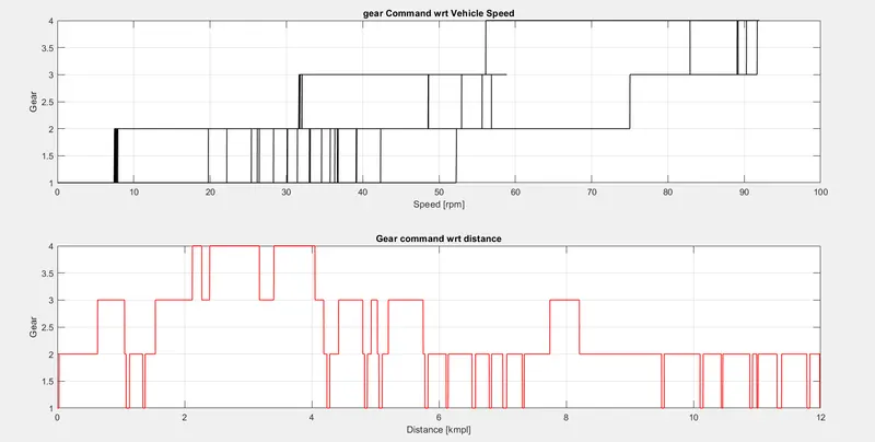
For HWFET drive cycle:

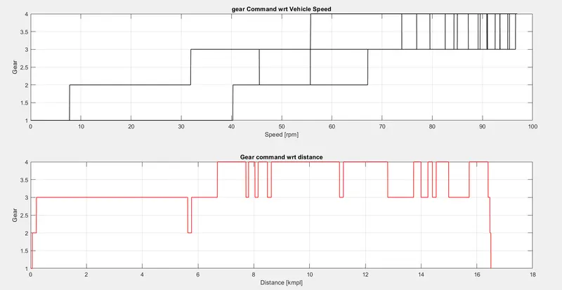
In those above graphs we can observe that, the gear shifting is required with respect to vehicle speed. Once the speed crosses the current gear maximum speed the gear shift is required to the next gear.

6. Plotting the Engine Fuel Consumption map:

For UDDS drive cycle:

For HWFET drive cycle: