Project 2 - Rankine cycle Simulator
Objective:
Power cycle: Converts heat energy by burning of fuel to shaft work i which a fluid working repeatedly performs a successsion of processes.
`sum`(cycle) Q(net) = `sum`W (net)
Q1-Q2 = W(T) - W(P)
Q1 = heat is transferred to working fluid
Q2 = heat rejected from the working fluid
W(P) = work is transferred to the working fluid
W(T) = work is transferred from the working fluid
Rankine Cycle: A reversible constant pressure heating process of water to form steam for steam boiler.
- For turbine ideal process would be a reversible adiabatic expansion of steam.
- For the condenser it would be a reversible constant pressure heat rejection as the steam condenses till it becomes saturated liquid &
- For the pump, ideal process would be a reversible adiabatic compression of this liquid ending at initial pressure.
Processes in a Rankine Cycle:
- Process 1-2: The working fluid is pumped from low to high pressure. As the fluid is a liquid at this stage, the pump requires little input energy.
- Process 2-3: The high-pressure liquid enters a boiler, where it is heated at a constant pressure by an external heat source to become a dry saturated vapour. The input energy required can be easily calculated graphically, using an enthalpy-entropy chart or Mollier diagram, or numerically using steam tables.
- Process 3-4: The dry saturated vapour expands through a turbine, generating power. This decreases the temperature and pressure of the vapour, and some condensation may occur.
- Process 4-1: The wet vapour then enters a condenser, where it is condensed at a constant pressure to become a saturated liquid.
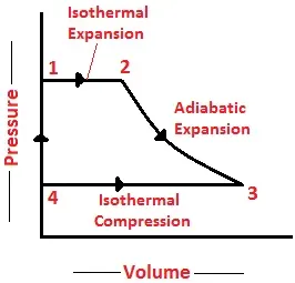 P-V Diagram
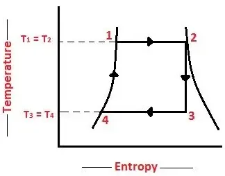 T-S Diagram
Procedure:
- Using a standard Xsteam library to get the steam table data for water. It must be used to calculate the points in between the state variables.
- The user inputs that have to be entered in command window are:
Pressure at the turbine inlet(in bar).
Temperature at the Inlet(in Degree Celcius).
Pressure at the condenser(in bar).
- Based on the inputs we will calculate state variables by using the equation of state and X_steam library which is a steam table and we can directly read values of state variables using it.
- After calculating the state variables at each state point we have calculated the turbine and pump work done.
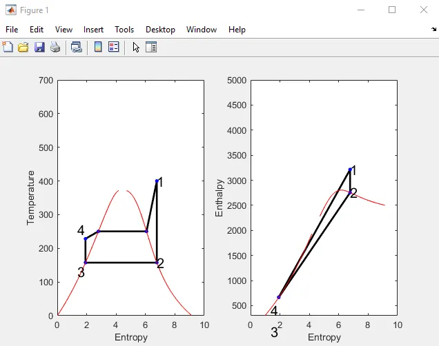
- At the end, we plotted the corresponding T-S and H-S plots for the given inputs.
MATLAB Code:
clear all
close all
clc
% Simulation Rankine cycle
% Process description
fprintf('1-2 Isobaric heat transfer\n')
fprintf('2-3 Isentropic Expansion\n')
fprintf('3-4 Isobaric heat rejection\n')
fprintf('4-1 Isentropic Compression\n')

% Inputs
p1 = input('Enter the pressure at the turbine Inlet(in bar):');
t1 = input('Enter the temperature at the Inlet(in Degree Celcius):');
p2 = input('Enter the Pressure at Condenser(in bar)');

% Input Conditions
t = XSteam('Tsat_p',p1);
if t1>=t
    h1 = XSteam('h_pT',p1,t1);
    s1 = XSteam('s_pT',p1,t1);
    % State points Evaluation
    p4 = p1;
    p3 = p2;
    h3 = XSteam('hL_p',p3);
    s3 = XSteam('sL_p',p3);
    t3 = XSteam('Tsat_p',p3);
    s2 = s1;
    t2 = t3;
    sf2 = XSteam('sL_p',p2);
    sg2 = XSteam('sV_p',p2);
    x2 = (s2 - sf2)/(sg2 - sf2);
    hf2 = XSteam('hL_p',p2);
    hg2 = XSteam('hV_p',p2);
    h2 = hf2 + x2*(hg2 - hf2);
    s4 = s3;
    h4 = XSteam('h_ps',p4,s4);
    cp4 = XSteam('Cp_ps',p4,s4);
    cv4 = XSteam('Cv_ps',p4,s4);
    g4 = cp4/cv4;
    o = (g4 - 1)/g4;
    t4 = t3*((p4/p3)^o);

    % Turbine & Pump Work
    wt = h1 - h2;
    wp = h4 - h3;
    % net work
    wnet = wt - wp;
    % Heat Supplied
    qs = h1 - h4;
    % Efficiency
    n_per = (wnet/qs)*100;
    % Steam rate per second
    stm_rate = 3600/(wt - wp);

    % For process 4-1, which is isobaric we use the expression dH=Cp*dT
    t5 = XSteam('Tsat_p',p1);
    s5 = XSteam('sL_p',p1);
    s6 = XSteam('sV_p',p1);
    % Output
    fprintf('\n\tRESULT\n')
    fprintf('At State point 1:\nP1 is :%4.2f Bar\nT1 is : %4.2f Degree Celcus \nH1 is :%4.2f kJ/kg\nS1 is :%4.2f kj/kgk\n\n',p1,t1,h1,s1)
    fprintf('At State point 2:\nP2 is :%4.2f Bar\nT2 is : %4.2f Degree Celcus \nH2 is :%4.2f kJ/kg\nS2 is :%4.2f kj/kgk\n\n',p2,t2,h2,s2)
    fprintf('At State point 3:\nP3 is :%4.2f Bar\nT3 is : %4.2f Degree Celcus \nH3 is :%4.2f kJ/kg\nS3 is :%4.2f kj/kgk\n\n',p3,t3,h3,s3)
    fprintf('At State point 4:\nP4 is :%4.2f Bar\nT4 is : %4.2f Degree Celcus \nH4 is :%4.2f kJ/kg\nS4 is :%4.2f kj/kgk\n\n',p4,t4,h4,s4)
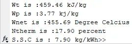
    fprintf('Wt is :%4.2f kJ/kg\nWp is :%4.2f kj/kg\nWnet is :%4.2f Degree Celcius\nNtherm is :%4.2f percent\nS.S.C is : %4.2f kg/kWh',wt,wp,wnet,n_per,stm_rate)

    % Vapour line
    temp = linspace(1,400,100);
    for i=1:length(temp)
        ent_1(i) = XSteam('sL_T',temp(i));
        ent_v(i) = XSteam('sV_T',temp(i));
        enth_1(i) = XSteam('hL_T',temp(i));
        enth_v(i) = XSteam('hV_T',temp(i));
    end
    % Plotting
    subplot(1,2,1)
    plot([s1 s2 s3 s4 s5 s6 s1],[t1 t2 t3 t4 t5 t5 t1],'color','k','linewidth',2,'marker','o','markersize',2,'markerfacecolor','b','markeredgecolor','b')
    hold on
    plot(ent_1,temp,'color','r')
    plot(ent_v,temp,'color','r')
    axis([0 10 0 700])
    text(s1,t1,'1','FontSize',15)
    text(s2,t2,'2','FontSize',15)
    text(s3,t3,'3','FontSize',15,'HorizontalAlignment','right','VerticalAlignment','top')
    text(s4,t4,'4','FontSize',15,'HorizontalAlignment','right','VerticalAlignment','bottom')
    xlabel('Entropy')
    ylabel('Temperature')
    subplot(1,2,2)
    plot([s1 s2 s3 s4 s1],[h1 h2 h3 h4 h1],'color','k','linewidth',2,'marker','o','markersize',2,'markerfacecolor','b','markeredgecolor','b')
    axis([0 10 300 5000])
    hold on
    plot(ent_v,enth_v,'color','r')
    plot(ent_1,enth_1,'color','r')
    text(s1,h1,'1','FontSize',15)
    text(s2,h2,'2','FontSize',15)
    text(s3,t3,'3','FontSize',15,'HorizontalAlignment','right','VerticalAlignment','top')
    text(s4,t4,'4','FontSize',15,'HorizontalAlignment','right','VerticalAlignment','bottom')
    xlabel('Entropy')
    ylabel('Enthalpy')

else
    fprintf('Enter Temperature Greater or Equal to Saturation Temperature')
end
OUTPUT:
User Input:

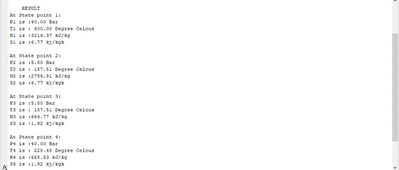
RESULTS:
T-S & H-S Plot