Challenge

Project 2 - Rankine cycle Simulator

AAmal Jacob5 Feb 2021

MATLAB

Rankine Cycle Simulator

Aim :- Create a code for Rankine Cycle Simulator using MATLAB

Objectives :-

1) The code should find the state points of rankine cycle based on user inputs

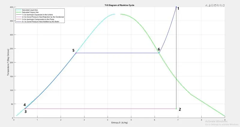
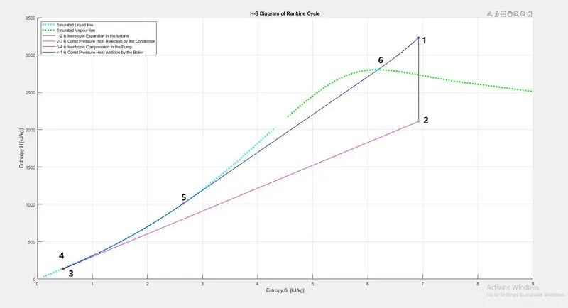
2) Plot the T-S and H-S diagram based on the inputs that we have given.

Theory :-

Rankine Cycle

The Rankine cycle is a model used to predict the performance of steam turbine systems. It was also used to study the performance of reciprocating steam engines. The Rankine cycle is an idealized Thermodynamic cycle of a heat engine that converts heat into mechanical work while undergoing phase change. It is an idealized cycle in which friction losses in each of the four components are neglected. The heat is supplied externally to a closed loop, which usually uses water as the working fluid.

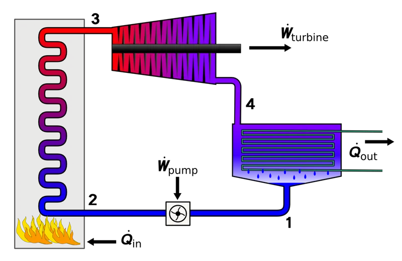
Physical layout of a Rankine cycle ;-

1.Pump

2.Boiler

3.Turbine

4.Condenser

Four Porcess of a Rankine cycle :-

Process 1-2 : The working fluid (here water) is pumped to the boiler. The pump converts the low pressure liquid to high pressure. As there is no entropy change this process is also called Isentropic compression.

Process 2-3 : Here the high pressure liquid is entered into a boiler where it is heated by an external source at constant pressure get converts to dry saturated vapour. This process is Constant pressure heat addition.

Process 3-4 : When the high temperature high pressure vapour enters the turbine the vapour expand and generate power. This reduces the pressure and temperature of the vapour. This process is called Isentropic expansion

Process 4-1 : The low pressure and temperature vapour will enter the condenser in this part and the vapour will get converted into saturated liquid at constant pressure, so this process is also called Constant pressure heat rejection.

Equations Used :-

P1 = Condenser Pressure

P2 = Pump pressure

P3 = Boiler pressure

P4 = Turbine Pressure

P1 = P4 , From process 4-1 we can see that the pressure is constant and only heat is rejected at condenser.

P2 = P3 , From process 2-3 we can see that the pressure is constant and heat is added at boiler.

S1= S2 , From process 1-2 we can see that the process is Isentropic compression.

S3 = S4 , From process 3-4 we can see that the process is Isentropic expansion.

h1, h2, h3, h4 = The specific enthalpies at state points.

s1, s2, s3, s4 = Entropies at state points

W = Mechanical power consumed by or provided to the system

Wt = Work done by the turbine

= h1 - h2

Wp = Work done by the turbine

= h4 - h3

Wnet = Wt - Wp

Q = Heat flow rate

Qin = h1- h4

Qout = h2- h3

Ntherm = Thermodynamic efficiency of the process

= Wnet/Qin

S.S.C = Specific Steam Consuption

= 3600/Wnet

Code Explanation :-

clear all
close all
clc

fprintf('         RANKINE CYCLE SIMULATOR\n');
fprintf('\n')

fprintf('1-2 is Isentropic Expansion in the turbine\n',1);
fprintf('2-3 is Const Pressure Heat Rejection by the Condenser\n');
fprintf('3-4 is Isentropic Compression in the Pump\n');
fprintf('4-1 is Const Pressure Heat Addition by the Boiler\n');
fprintf('\n')
p1 = input('Enter the Pressure at the Turbine Inlet(in bar): ');
t1 = input('Enter the Temperature at the Turbine Inlet(in Degree Celcius): ');
p2 = input('Enter the Pressure at condenser(in bar): ');
fprintf('\n')

fprintf('         RESULTS\n');
fprintf('\n')



% At state point 1
h1= XSteam('h_pT',p1,t1);
s1= XSteam('s_ph',p1,h1);

fprintf('At state point 1\n');
fprintf('P1 is :%f Bar\n',p1);
fprintf('T1 is :%f Deg Celcius\n',t1);
fprintf('H1 is :%f kJ/kg\n',h1);
fprintf('S1 is :%f kJ/kgK\n',s1);
fprintf('\n')

% At state point 2
s2=s1;
t2= XSteam('T_ps',p2,s2);
% S1=S2
% S2= Sf + (x*Sfg)
% x= (S2-Sf)/Sfg
sf2 = XSteam('sL_p',p2);
sg2= XSteam('sV_p',p2);
sfg2=sg2-sf2;
x2= (s2-sf2)/sfg2;

hf2=XSteam('hL_p',p2);
hg2=XSteam('hV_p',p2);
hfg2=hg2-hf2;
h2=hf2+(x2*hfg2);

fprintf('At state point 2\n');
fprintf('P2 is :%f Bar\n',p2);
fprintf('T2 is :%f Deg Celcius\n',t2);
fprintf('H2 is :%f kJ/kg\n',h2);
fprintf('S2 is :%f kJ/kgK\n',s2);
fprintf('X2 is :%f \n',x2);
fprintf('\n')

% At state point 3
p3=p2;
s3=XSteam('sL_p',p3);
t3=XSteam('Tsat_p',p3);
h3=XSteam('hL_p',p3);
fprintf('At state point 3\n');
fprintf('P3 is :%f Bar\n',p3);
fprintf('T3 is :%f Deg Celcius\n',t3);
fprintf('H3 is :%f kJ/kg\n',h3);
fprintf('S3 is :%f kJ/kgK\n',s3);
fprintf('\n')

% At state point 4
p4=p1;
s4=s3;
t4=XSteam('T_ps',p4,s4);
h4=XSteam('h_ps',p4,s4);
fprintf('At state point 4\n');
fprintf('P4 is :%f Bar\n',p4);
fprintf('T4 is :%f Deg Celcius\n',t4);
fprintf('H4 is :%f kJ/kg\n',h4);
fprintf('S4 is :%f kJ/kgK\n',s4);

% At state point 5
p5=p1;
s5=XSteam('sL_p',p5);
t5=XSteam('Tsat_p',p5);
h5=XSteam('hL_p',p5);

% At state point 6
p6=p1;
t6=XSteam('Tsat_p',p6);
s6=XSteam('sV_p',p6);
h6=XSteam('hV_p',p6);

%Calculating Wt,Wp,Wnet,Qin,Qout,Ntherm and SSC
Wt=h1-h2;
Wp=h4-h3;
Wnet=Wt-Wp;
Qin=h1-h4;
Qout=h2-h3;
Ntherm=Wnet/Qin;
SSC=3600/Wnet;

fprintf('\n')
fprintf('Wt is :%f kJ/kg\n',Wt);
fprintf('Wp is :%f kJ/kg\n',Wp);
fprintf('Wnet is :%f kJ/kg\n',Wnet);
fprintf('Ntherm is :%f Percent\n',Ntherm);
fprintf('S.S.C is :%f kg/kWh\n',SSC);

%ploting T-S diagram

figure(1)
hold on
%Plotting the saturation curve in T-S diagram
p=linspace(0.01,220,400);
for i=1:length(p)
    sl(i)=XSteam('sL_p',p(i));
    hl(i)=XSteam('hL_p',p(i));
    tl(i)=XSteam('Tsat_p',p(i));
    sg(i)=XSteam('sV_p',p(i));
    hg(i)=XSteam('hV_p',p(i));
    tg(i)=XSteam('Tsat_p',p(i));
end
grid on
plot (sl,tl,':','linewidth',3,'color','c')
plot (sg,tg,':','linewidth',3,'color','g')

% Ploting Curves connecting state points in T-S diagram
plot([s1 s2],[t1 t2],'linewidth',1,'color','k');
plot([s2 s3],[t2 t3],'linewidth',1,'color','m');
plot([s3 s4],[t3 t4],'linewidth',1,'color','r');

PC1=linspace(p4,p5,400);
TC1=linspace(t4,t5,400);
for i=1:length(TC1)
SC1(i)=XSteam('s_pT',PC1(i),TC1(i));
end
plot(SC1,TC1,'linewidth',1,'color','b');

plot([s5 s6],[t5 t6],'linewidth',1,'color','b');

PC2=linspace(p6,p1,400);
TC2=linspace(t6,t1,400);
for i=1:length(TC2)
SC2(i)=XSteam('s_pT',PC2(i),TC2(i));
end
plot(SC2,TC2,'linewidth',1,'color','b');

% Marking each state points 
plot (s1,t1,'*','color','b')
plot (s2,t2,'*','color','g')
plot (s3,t3,'*','color','black')
plot (s4,t4,'*','color','r')
plot (s5,t5,'*','color','m')
plot (s6,t6,'*','color','c')


% Giving Title,labels and legend
title('T-S Diagram of Rankine Cycle')
xlabel('Entropy,S  [kJ/kg]')
ylabel('Temperature,T [Deg Celcius]')
legend('Saturated Liquid line','Saturated Vapour line','1-2 is Isentropic Expansion in the turbine','2-3 is Const Pressure Heat Rejection by the Condenser','3-4 is Isentropic Compression in the Pump','4-1 is Const Pressure Heat Addition by the Boiler','location','northwest')
hold off

%ploting H-S diagram

figure(2)
hold on
%Plotting the saturation curve in H-S diagram
p=linspace(0.01,220,400);
for i=1:length(p)
    sl(i)=XSteam('sL_p',p(i));
    hl(i)=XSteam('hL_p',p(i));
    tl(i)=XSteam('Tsat_p',p(i));
    sg(i)=XSteam('sV_p',p(i));
    hg(i)=XSteam('hV_p',p(i));
    tg(i)=XSteam('Tsat_p',p(i));
end
grid on
plot (sl,hl,':','linewidth',3,'color','c')
plot (sg,hg,':','linewidth',3,'color','g')

% Ploting Curves connecting state points in H-S diagram
plot([s1 s2],[h1 h2],'linewidth',1,'color','k')

PC3=linspace(p2,p3,400);
HC3=linspace(h2,h3,400);
for i=1:length(PC3)
SC3(i)=XSteam('s_ph',PC3(i),HC3(i));
end
plot(SC3,HC3,'linewidth',1,'color','m')

plot([s3 s4],[h3 h4],'linewidth',1,'color','r')

PC4=linspace(p4,p5,400);
HC4=linspace(h4,h5,400);
for i=1:length(PC4)
SC4(i)=XSteam('s_ph',PC4(i),HC4(i));
end
plot(SC4,HC4,'linewidth',1,'color','b')

PC5=linspace(p5,p6,400);
HC5=linspace(h5,h6,400);
for i=1:length(PC5)
SC5(i)=XSteam('s_ph',PC5(i),HC5(i));
end
plot(SC5,HC5,'linewidth',1,'color','b')

PC6=linspace(p6,p1,400);
HC6=linspace(h6,h1,400);
for i=1:length(PC6)
SC6(i)=XSteam('s_ph',PC6(i),HC6(i));
end
plot(SC6,HC6,'linewidth',1,'color','b')

% Marking each state points 
plot (s1,h1,'*','color','b')
plot (s2,h2,'*','color','g')
plot (s3,h3,'*','color','black')
plot (s4,h4,'*','color','r')
plot (s5,h5,'*','color','m')
plot (s6,h6,'*','color','c')
hold off

% Giving Title,labels and legend
title('H-S Diagram of Rankine Cycle')
xlabel('Entropy,S  [kJ/kg]')
ylabel('Enthalpy,H [kJ/kg]')
legend('Saturated Liquid line','Saturated Vapour line','1-2 is Isentropic Expansion in the turbine','2-3 is Const Pressure Heat Rejection by the Condenser','3-4 is Isentropic Compression in the Pump','4-1 is Const Pressure Heat Addition by the Boiler','location','northwest')

1) "clear all, close all, clc " they are used to clear all the previous programs data and to begin as fresh.

2) Things that comes after "%" symbol are just comments , they dont have any influnce on the program.

3) The below steps are just to print things that are given in single quotes

fprintf(' RANKINE CYCLE SIMULATOR\n');
fprintf('\n')

fprintf('1-2 is Isentropic Expansion in the turbine\n',1);
fprintf('2-3 is Const Pressure Heat Rejection by the Condenser\n');
fprintf('3-4 is Isentropic Compression in the Pump\n');
fprintf('4-1 is Const Pressure Heat Addition by the Boiler\n');
fprintf('\n')

4) The below given codes will ask for user inputs and will save the inputed values in the respected variables
p1 = input('Enter the Pressure at the Turbine Inlet(in bar): ');
t1 = input('Enter the Temperature at the Turbine Inlet(in Degree Celcius): ');
p2 = input('Enter the Pressure at condenser(in bar): ');
fprintf('\n')

fprintf(' RESULTS\n');
fprintf('\n')

5) We give the P1 , P2 and T1 in the above steps

6) Now we need to find the rest of the state point 1 Values, which we will get from the XSteam code

XSteam function act as our steam table

As the temperature is 400 deg Celcius the vapour is now super heated condition.

h1= XSteam('h_pT',p1,t1); =We have p1 and t1 so we get the value of h1 from Xsteam, as a funtion of p1 and t1
s1= XSteam('s_ph',p1,h1); =Now we have p1, t1 and h1 so we get the value of s1 from Xsteam, as a funtion of p1 and h1

fprintf('At state point 1\n');
fprintf('P1 is :%f Bar\n',p1);
fprintf('T1 is :%f Deg Celcius\n',t1);
fprintf('H1 is :%f kJ/kg\n',h1);
fprintf('S1 is :%f kJ/kgK\n',s1);
fprintf('\n') = The above steps are just to print the values of P,T,H and S with its units in command window

7) From state point 1 we got s1 and we know the p2. From that we can find the state point 2 values
s2=s1;
t2= XSteam('T_ps',p2,s2); = We get t2 from Xsteam as we have the p2 and s2

% S1=S2
% S2= Sf + (x*Sfg)
% x= (S2-Sf)/Sfg = x is the dryness fraction, The term dryness fraction is related with wet steam. It is defined as the ratio of the mass of actual steam to the mass of steam containing it. It is usuallyexpressed by the symbol 'x'

Sf is the entropy value for the p2 on saturation liquid curve

Sg is the entopy value for the p2 on saturation vapour curve

Sfg is sf- sg

sf2 = XSteam('sL_p',p2);
sg2= XSteam('sV_p',p2); = sf2 and sg2 we take there values from Xsteam with respect to p2
sfg2=sg2-sf2;
x2= (s2-sf2)/sfg2; = Using the equation given above we calculate the dryness fraction.

Hf is the enthalpy value for the p2 on saturation liquid curve

Hg is the enthalpy value for the p2 on saturation vapour curve

Hfg is hf- hg

hf2=XSteam('hL_p',p2);
hg2=XSteam('hV_p',p2); = hf2 and hg2 we take there values from Xsteam with respect to p2.
hfg2=hg2-hf2;
h2=hf2+(x2*hfg2); = We have already calculated the value of X2 so with that we can calculate the value of h2

fprintf('At state point 2\n');
fprintf('P2 is :%f Bar\n',p2);
fprintf('T2 is :%f Deg Celcius\n',t2);
fprintf('H2 is :%f kJ/kg\n',h2);
fprintf('S2 is :%f kJ/kgK\n',s2);
fprintf('X2 is :%f \n',x2);
fprintf('\n') = The above steps are just to print the values of P,T,H and S with its units in command window

8) For state point 3, We have p3 and we know the point is on saturation line, soo..

p3=p2;
s3=XSteam('sL_p',p3); = s3=sf, or we can take the value from Xsteam as a funtion of pressure.
t3=XSteam('Tsat_p',p3); = we get t3 as a funtion of p3 in saturated condition.
h3=XSteam('hL_p',p3); = we get the h3 as a funtion of p3 in saturated condition.
fprintf('At state point 3\n');
fprintf('P3 is :%f Bar\n',p3);
fprintf('T3 is :%f Deg Celcius\n',t3);
fprintf('H3 is :%f kJ/kg\n',h3);
fprintf('S3 is :%f kJ/kgK\n',s3);
fprintf('\n') = The above steps are just to print the values of P,T,H and S with its units in command window.

9) For state point 4, We have p4, s4 so we can calculate others with that.

p4=p1;
s4=s3;
t4=XSteam('T_ps',p4,s4); = t4 can be taken from Xsteam as a funtion of p4 and s4
h4=XSteam('h_ps',p4,s4); = h4 can be taken from Xsteam as a funtion of p4 and s4
fprintf('At state point 4\n');
fprintf('P4 is :%f Bar\n',p4);
fprintf('T4 is :%f Deg Celcius\n',t4);
fprintf('H4 is :%f kJ/kg\n',h4);
fprintf('S4 is :%f kJ/kgK\n',s4); = The above steps are just to print the values of P,T,H and S with its units in command window.

10) The state point 5 is on the saturation line so it is easy to get the values from the Xsteam with respect to p5

p5=p1;
s5=XSteam('sL_p',p5);
t5=XSteam('Tsat_p',p5);
h5=XSteam('hL_p',p5);

11) The state point 6 is also on the saturation line so it is easy to get the values from the Xsteam with respect to p6

p6=p1;
t6=XSteam('Tsat_p',p6);
s6=XSteam('sV_p',p6);
h6=XSteam('hV_p',p6);

12) Now we have all the values of H, S, T, P at every state points so we can calculate Wt,Wp,Wnet,Qin,Qout,Ntherm and SSC
Wt=h1-h2;
Wp=h4-h3;
Wnet=Wt-Wp;
Qin=h1-h4;
Qout=h2-h3;
Ntherm=Wnet/Qin;
SSC=3600/Wnet;

now print the values in the command window

fprintf('\n')
fprintf('Wt is :%f kJ/kg\n',Wt);
fprintf('Wp is :%f kJ/kg\n',Wp);
fprintf('Wnet is :%f kJ/kg\n',Wnet);
fprintf('Ntherm is :%f Percent\n',Ntherm);
fprintf('S.S.C is :%f kg/kWh\n',SSC);

13) Finding every state points and its values and we have calculated the outputs, so now we can plot T-S diagram.

figure(1)
hold on
14) For plotting the saturation curve in T-S diagram, we take the lowest value of pressure and the peak value of pressure. Then start a for loop for getting sl,hl,tl,sg,hg,tg at every point of pressure.
p=linspace(0.01,220,400); = takeing the pressure range and divide that into 400 equal parts
for i=1:length(p) = for the length of p calculate values for each sl,hl,tl,sg,hg,tg
sl(i)=XSteam('sL_p',p(i));
hl(i)=XSteam('hL_p',p(i));
tl(i)=XSteam('Tsat_p',p(i));
sg(i)=XSteam('sV_p',p(i));
hg(i)=XSteam('hV_p',p(i));
tg(i)=XSteam('Tsat_p',p(i));
end
grid on
plot (sl,tl,':','linewidth',3,'color','c') = This is to plot the saturated liquid curve
plot (sg,tg,':','linewidth',3,'color','g') = This is to plot the saturated vapour curve

15) Now we can plot Curves connecting state points in T-S diagram

s1-s2,s2-s3,s3-s4 are straight lines so we used the formula below
plot([s1 s2],[t1 t2],'linewidth',1,'color','k');
plot([s2 s3],[t2 t3],'linewidth',1,'color','m');
plot([s3 s4],[t3 t4],'linewidth',1,'color','r');

but the s4-s5 and s6-s1 are curve so we used the formula below.

we divide the pressure value and time , then put that pressure and temperature to find s value at each points, then we get a curve by connecting these values

PC1=linspace(p4,p5,400);
TC1=linspace(t4,t5,400);
for i=1:length(TC1)
SC1(i)=XSteam('s_pT',PC1(i),TC1(i));
end
plot(SC1,TC1,'linewidth',1,'color','b');

plot([s5 s6],[t5 t6],'linewidth',1,'color','b'); = s5-s6 is straight line so we used this

Again we need a curve for s6-s1 so we used the code below

PC2=linspace(p6,p1,400);
TC2=linspace(t6,t1,400);
for i=1:length(TC2)
SC2(i)=XSteam('s_pT',PC2(i),TC2(i));
end
plot(SC2,TC2,'linewidth',1,'color','b');

16) To mark each state points we give a marker there
plot (s1,t1,'*','color','b')
plot (s2,t2,'*','color','g')
plot (s3,t3,'*','color','black')
plot (s4,t4,'*','color','r')
plot (s5,t5,'*','color','m')
plot (s6,t6,'*','color','c')

17) Giving Title,labels and legend to make the graph more readable
title('T-S Diagram of Rankine Cycle')
xlabel('Entropy,S [kJ/kg]')
ylabel('Temperature,T [Deg Celcius]')
legend('Saturated Liquid line','Saturated Vapour line','1-2 is Isentropic Expansion in the turbine','2-3 is Const Pressure Heat Rejection by the Condenser','3-4 is Isentropic Compression in the Pump','4-1 is Const Pressure Heat Addition by the Boiler','location','northwest')
hold off

18) Now we can plot the H-S diagram

figure(2)
hold on
19) As we done for the T-SP here also we plot the saturation curve in H-S diagram, Same procedure is followed
p=linspace(0.01,220,400);
for i=1:length(p)
sl(i)=XSteam('sL_p',p(i));
hl(i)=XSteam('hL_p',p(i));
tl(i)=XSteam('Tsat_p',p(i));
sg(i)=XSteam('sV_p',p(i));
hg(i)=XSteam('hV_p',p(i));
tg(i)=XSteam('Tsat_p',p(i));
end
grid on
plot (sl,hl,':','linewidth',3,'color','c')
plot (sg,hg,':','linewidth',3,'color','g')

20) After that we can plot Curves connecting state points in H-S diagram. This is also same as the T-S diagrams procedure.

plot([s1 s2],[h1 h2],'linewidth',1,'color','k')

PC3=linspace(p2,p3,400);
HC3=linspace(h2,h3,400);
for i=1:length(PC3)
SC3(i)=XSteam('s_ph',PC3(i),HC3(i));
end
plot(SC3,HC3,'linewidth',1,'color','m')

plot([s3 s4],[h3 h4],'linewidth',1,'color','r')

PC4=linspace(p4,p5,400);
HC4=linspace(h4,h5,400);
for i=1:length(PC4)
SC4(i)=XSteam('s_ph',PC4(i),HC4(i));
end
plot(SC4,HC4,'linewidth',1,'color','b')

PC5=linspace(p5,p6,400);
HC5=linspace(h5,h6,400);
for i=1:length(PC5)
SC5(i)=XSteam('s_ph',PC5(i),HC5(i));
end
plot(SC5,HC5,'linewidth',1,'color','b')

PC6=linspace(p6,p1,400);
HC6=linspace(h6,h1,400);
for i=1:length(PC6)
SC6(i)=XSteam('s_ph',PC6(i),HC6(i));
end
plot(SC6,HC6,'linewidth',1,'color','b')

21) Using belows code we can mark each state points
plot (s1,h1,'*','color','b')
plot (s2,h2,'*','color','g')
plot (s3,h3,'*','color','black')
plot (s4,h4,'*','color','r')
plot (s5,h5,'*','color','m')
plot (s6,h6,'*','color','c')
hold off

22) Giving Title,labels and legend

title('H-S Diagram of Rankine Cycle')
xlabel('Entropy,S [kJ/kg]')
ylabel('Enthalpy,H [kJ/kg]')
legend('Saturated Liquid line','Saturated Vapour line','1-2 is Isentropic Expansion in the turbine','2-3 is Const Pressure Heat Rejection by the Condenser','3-4 is Isentropic Compression in the Pump','4-1 is Const Pressure Heat Addition by the Boiler','location','northwest')

Results :-

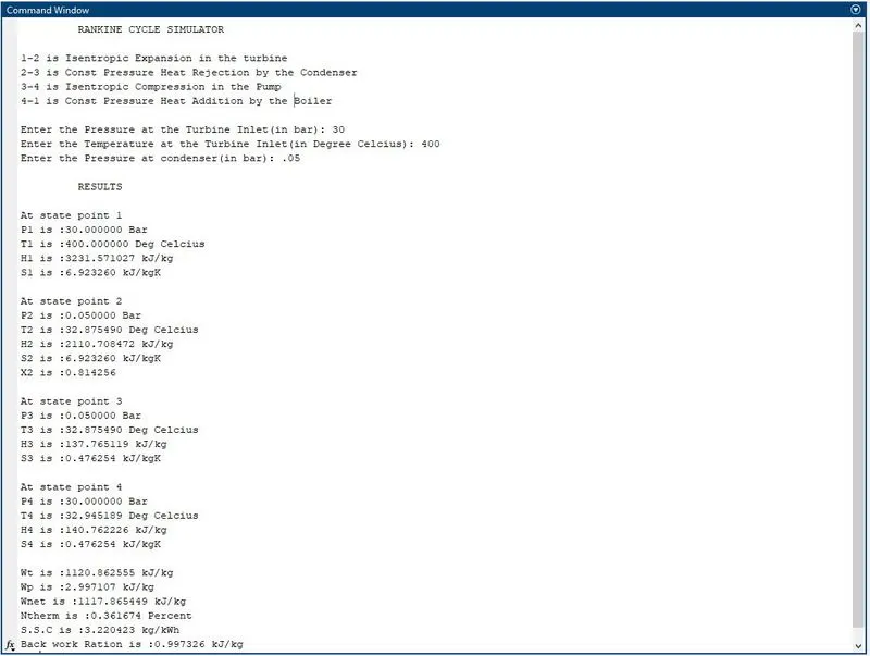
1) The figure below shows all the results and values of the state points