Project 2 - Rankine cycle Simulator
Project : 2 Rankine cycle Simulator
Abstract
These project is regarding MATLAB code for determining state points parameters of Rankine Cycle Simulator in relation to user inputs and additionally plotting T-S and H-S plots. The theory about Rankine cycle simulator working is explained and finally Net work output, work ratio and the thermal efficiency are also calculated
Theory
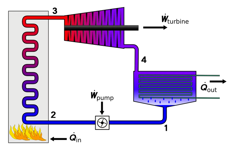
The Rankine cycle or Rankine Vapor Cycle is the process widely used by power plants such as coal-fired power plants or nuclear reactors. In this mechanism, a fuel is used to produce heat within a boiler, converting water into steam which then expands through a turbine producing useful work. This is a thermodynamic cycle which converts heat into mechanical energy—which usually gets transformed into electricity by electrical generation.
Ideal Rankine Cycle
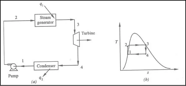
There are four processes in the Rankine cycle.
- Process 1–2: The working fluid is pumped from low to high pressure. As the fluid is a liquid at this stage, the pump requires little input energy.
In other words Process 1-2 is [Isentropic compression]
- Process 2–3: The high-pressure liquid enters a boiler, where it is heated at constant pressure by an external heat source to become a dry saturated vapour. The input energy required can be easily calculated graphically, using an enthalpy–entropy chart (h–s chart, or Mollier diagram), or numerically, using steam tables.
In other words Process 2-3 is [Constant pressure heat addition in boiler]
- Process 3–4: The dry saturated vapour expands through a turbine, generating power. This decreases the temperature and pressure of the vapour, and some condensation may occur. The output in this process can be easily calculated using the chart or tables noted above.
In other words Process 3-4 is [Isentropic expansion]
- Process 4–1: The wet vapour then enters a condenser, where it is condensed at a constant pressure to become a saturated liquid.
In other words Process 4-1 is [Constant pressure heat rejection in condenser]
In an ideal Rankine cycle the pump and turbine would be isentropic, i.e., the pump and turbine would generate no entropy and hence maximize the net work output. Processes 1–2 and 3–4 would be represented by vertical lines on the T–s diagram and more closely resemble that of the Carnot cycle. The Rankine cycle shown here prevents the state of the working fluid from ending up in the superheated vapor region after the expansion in the turbine, which reduces the energy removed by the condensers.
The actual vapor power cycle differs from the ideal Rankine cycle because of irreversibilities in the inherent components caused by fluid friction and heat loss to the surroundings; fluid friction causes pressure drops in the boiler, the condenser, and the piping between the components, and as a result the steam leaves the boiler at a lower pressure; heat loss reduces the net work output, thus heat addition to the steam in the boiler is required to maintain the same level of net work output.
Real Rankine cycle (non-ideal)
In a real power-plant cycle (the name "Rankine" cycle is used only for the ideal cycle), the compression by the pump and the expansion in the turbine are not isentropic. In other words, these processes are non-reversible, and entropy is increased during the two processes. This somewhat increases the power required by the pump and decreases the power generated by the turbine.
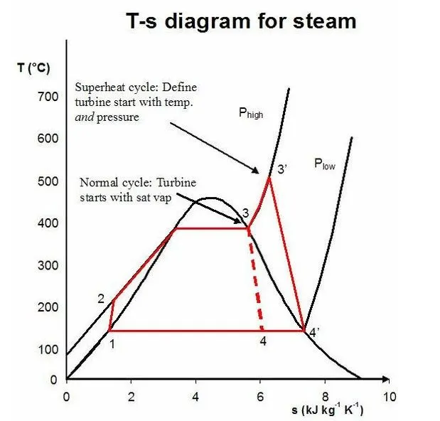
In particular, the efficiency of the steam turbine will be limited by water-droplet formation. As the water condenses, water droplets hit the turbine blades at high speed, causing pitting and erosion, gradually decreasing the life of turbine blades and efficiency of the turbine. The easiest way to overcome this problem is by superheating the steam. On the T–s diagram above, state 3 is at a border of the two-phase region of steam and water, so after expansion the steam will be very wet. By superheating, state 3 will move to the right (and up) in the diagram and hence produce a drier steam after expansion.
Application of the First law of thermodynamics to the control volume (pump, steam generator, turbine and condenser), gives
Work done on pump, per kg of water, WP= h2-h1
Energy added in steam generator, q1= h3-h2
Work delivered by turbine, WT= h3-h4
Energy rejected in the condenser, q2= h4-h1
Net work done, Wnet = Wt-Wp
The thermal efficiency of the Rankine cycle is given by,

MATLAB code
clear all
close all
clc

disp ('     RANKINE CYCLE SIMULATOR   ');
disp('1-2 is Isentropic Expansion in the Turbine');
disp('2-3 is Const Pressure Heat Rejection by the condenser');
disp('3-4 is Isentropic compression in the Pumb');
disp('4-1 is Const Pressure Heat addition by the Boiler');

input_1 = input('Enter the pressure at the turbine inlet (in bar) : ');
input_2 = input('Enter the temperature at the turbine inlet (in Degree celcius) :');
input_3 = input('Enter the pressure at the condenser (in bar) : ');

%p2_turbine_outlet=p3_condenser_outlet
% p3_condenser_outlet=0.05;

%At state point : 1

s1 = XSteam('s_pT',input_1,input_2);
h1 = XSteam('h_pT',input_1,input_2);
v1 = XSteam('v_pT',input_1,input_2);

disp('At state point 1')
fprintf('P1 is :%f \n',input_1)
fprintf('T1 is :%f \n',input_2)
fprintf('H1 is :%f \n',h1)
fprintf('S1 is :%f \n\n',s1)

%At state point : 2

s2 = s1;

T2 = XSteam('T_ps',input_3,s2);
h2 = XSteam('h_ps',input_3,s2);
v2 = XSteam('v_ps',input_3,s2);

sf = XSteam('sL_p',input_3);
sg = XSteam('sV_p',input_3);
Sfg= sg-sf;
x = (s2-sf)/(Sfg);

hf = XSteam('hL_p',input_3);
hg = XSteam('hV_p',input_3);
Hfg= hg-hf;


disp('At state point 2')
fprintf('P2 is :%f \n',input_3)
fprintf('T2 is :%f \n',T2)
fprintf('H2 is :%f \n',h2)
fprintf('S2 is :%f \n',s2)
fprintf('X2 is :%f \n\n',x)

%At state point : 3

p3 = input_3;
h3 = hf;
T3 = XSteam('Tsat_p',p3);
s3 = XSteam('sL_p',p3);
v3 = XSteam('vL_p',p3,h3);

disp('At state point 3')
fprintf('P3 is :%f \n',p3)
fprintf('T3 is :%f \n',T3)
fprintf('H3 is :%f \n',h3)
fprintf('S3 is :%f \n\n',s3)

%At state point : 4

s4 = s3;
p4 = input_1;
T4 = XSteam('T_ps',p4,s4);
h4 =  XSteam('h_ps',p4,s4);
v4 =  XSteam('v_ps',p4,s4);

disp('At state point 4')
fprintf('P4 is :%f \n',p4)
fprintf('T4 is :%f \n',T4)
fprintf('H4 is :%f \n',h4)
fprintf('S4 is :%f \n\n',s4)

%At state point : 5
p5 = p4;
T5 =  XSteam('Tsat_p',p5);
s5 =  XSteam('sL_p',p5);
h5 =  XSteam('hL_p',p5);

disp('At state point 5')
fprintf('P5 is :%f \n',p5)
fprintf('T5 is :%f \n',T5)
fprintf('H5 is :%f \n',h5)
fprintf('S5 is :%f \n\n',s5)

%At state point : 6
p6 = p5;
T6 = XSteam('Tsat_p',p6);
s6 =  XSteam('sV_p',p6);
h6 =  XSteam('hV_p',p6);


disp('At state point 6')
fprintf('P6 is :%f \n',p6)
fprintf('T6 is :%f \n',T6)
fprintf('H6 is :%f \n',h6)
fprintf('S6 is :%f \n\n',s6)

Wt = h1-h2;
Wp = h4-h3;
Qin  = h1-h4;
Qout = h2-h3;

Wnet = Wt-Wp;          %Net Work done
Ntherm = (Wnet)/(Qin); %Thermal Efficency
SSC = 3600/Wnet ;      %Specific Steam conductivity

fprintf('Net Work done is :%f \n',Wnet)
fprintf('Thermal Efficency is :%f \n',Ntherm)
fprintf('Specific Steam conductivity is :%f \n',SSC)

%Plot the TS diagram
figure(1)
% 1 to 2
plot ([s1 s2],[input_2 T2],'linewidth',3)
hold on
% 2 to 3
plot ([s2 s3],[T2 T3],'linewidth',3)
% 3 to 4
plot ([s3 s4],[T3 T4],'linewidth',3)
% 4 to 5
tc1 = linspace(T4,T5,1000);
pc1 = linspace(p4,p5,1000);
for i=1:length(tc1)
    sc1(i) = XSteam('s_pT',pc1(i),tc1(i));
end
plot (sc1,tc1,'linewidth',3,'color','r')
% 5 to 6
plot ([s5 s6],[T5 T6],'linewidth',3)
% 6 to 1
tc2 = linspace(T6,input_2,1000);
pc2 = linspace(p6,input_1,1000);
for i=1:length(tc2)
    sc2(i) = XSteam('s_pT',pc2(i),tc2(i));
end
plot (sc2,tc2,'linewidth',3)
legend('Saturation Curve L','Saturation Curve V','Turbine','Condenser','pumb','Boiler','location','northwest')
xlabel('Entropy(S)')
ylabel('Temperature(T)')
title('T-S diagram')

%Saturation curve for TS
t = linspace(0,373.15,500);
for i= 1:length(t)
    %Saturated liquid line
    sL(i) = XSteam('sL_T',t(i));
    sV(i) = XSteam('sV_T',t(i));

end

plot(sL,t,'g')
hold on
plot(sV,t,'g')

%Plot the HS diagram

figure(2)

% 1 to 2
plot ([s1 s2],[h1 h2],'linewidth',3)
hold on

% 2 to 3
hc1 = linspace(h2,h3,1000);
pc3 = linspace(input_3,p3,1000);
for i=1:length(hc1)
    sc3(i) = XSteam('s_ph',pc3(i),hc1(i));
end
plot (sc3,hc1,'linewidth',3)

% 3 to 4
plot ([s3 s4],[h3 h4],'linewidth',3)

% 4 to 5
hc2 = linspace(h4,h5,1000);
pc4 = linspace(p4,p5,1000);
for i=1:length(hc2)
    sc4(i) = XSteam('s_ph',pc4(i),hc2(i));
end
plot (sc4,hc2,'linewidth',3)

% 5 to 6
hc3 = linspace(h5,h6,1000);
pc5 = linspace(p5,p6,1000);
for i=1:length(hc3)
    sc5(i) = XSteam('s_ph',pc5(i),hc3(i));
end
plot (sc5,hc3,'linewidth',3)

% 6 to 1
hc4 = linspace(h6,h1,1000);
pc6 = linspace(p6,input_1,1000);
for i=1:length(hc4)
    sc6(i) = XSteam('s_ph',pc6(i),hc4(i));
end
plot (sc6,hc4,'linewidth',3)

%Saturation curve for HS
 t2=linspace(0,input_2,1000);
 for j=1:length(t2)
     sl(j)=XSteam('sL_T',t2(j));
     sv(j)=XSteam('sV_T',t2(j));
     hl(j)=XSteam('hL_T',t2(j));
     hv(j)=XSteam('hV_T',t2(j));
end

plot(sl,hl)
hold on
plot(sv,hv)
legend('Saturation Curve L','Saturation Curve V','Turbine','Condenser','pumb','Boiler','location','northwest')
xlabel('Entropy(S)')
ylabel('Enthaply(H)')
title('H-S diagram')
Step wise explanation
clear all
close all
clc

disp ('     RANKINE CYCLE SIMULATOR   ');
disp('1-2 is Isentropic Expansion in the Turbine');
disp('2-3 is Const Pressure Heat Rejection by the condenser');
disp('3-4 is Isentropic compression in the Pumb');
disp('4-1 is Const Pressure Heat addition by the Boiler');

input_1 = input('Enter the pressure at the turbine inlet (in bar) : ');
input_2 = input('Enter the temperature at the turbine inlet (in Degree celcius) :');
input_3 = input('Enter the pressure at the condenser (in bar) : ');
The above commands are used to display the results in the command prompt and the user need to input the inlet temperature , inlet pressure and condenser pressure
%At state point : 1

s1 = XSteam('s_pT',input_1,input_2);
h1 = XSteam('h_pT',input_1,input_2);
v1 = XSteam('v_pT',input_1,input_2);

disp('At state point 1')
fprintf('P1 is :%f \n',input_1)
fprintf('T1 is :%f \n',input_2)
fprintf('H1 is :%f \n',h1)
fprintf('S1 is :%f \n\n',s1)
In this XSteam command is used in which it provides accurate data for water and steam and mixtures of water and steam properties from 0 - 1000 bar and from 0 - 2000 deg C. It is programmed as a matlab . m file
So with this command s1,h1,v1 is calculated with respect to the given pressure and temperature. This values are not in the saturated line so this s_pT, h_pT and v_pT command is used to derive the value from XSteam
In last fprintf comand is used to display the results
%At state point : 2

s2 = s1;

T2 = XSteam('T_ps',input_3,s2);
h2 = XSteam('h_ps',input_3,s2);
v2 = XSteam('v_ps',input_3,s2);

sf = XSteam('sL_p',input_3);
sg = XSteam('sV_p',input_3);
Sfg= sg-sf;
x = (s2-sf)/(Sfg);

hf = XSteam('hL_p',input_3);
hg = XSteam('hV_p',input_3);
Hfg= hg-hf;


disp('At state point 2')
fprintf('P2 is :%f \n',input_3)
fprintf('T2 is :%f \n',T2)
fprintf('H2 is :%f \n',h2)
fprintf('S2 is :%f \n',s2)
fprintf('X2 is :%f \n\n',x)
From 1 to 2 it is isentropic process in which entropy are constant. And also condenser pressure is given, so with repect to pressure and entropy T2, h2, v2 is derived from the Xsteam
And also Entropy and Enthalpy of the saturated line need to be caluculated for both vapour and fluid state. Entropy of fluid(sf), Entropy of vapour(sg) and mixture of fluid and vapour of entropy need to be calculated in order to get the Dryness fraction(x) value.
Similarly Enthalpy of fluid , gas and mixture of both are calculated using the same method.
And last all this values are displayed in the results using fprintf
%At state point : 3

p3 = input_3;
h3 = hf;
T3 = XSteam('Tsat_p',p3);
s3 = XSteam('sL_p',p3);
v3 = XSteam('vL_p',p3,h3);

disp('At state point 3')
fprintf('P3 is :%f \n',p3)
fprintf('T3 is :%f \n',T3)
fprintf('H3 is :%f \n',h3)
fprintf('S3 is :%f \n\n',s3)
In here h3=h4 its because h3 point is located in the saturated line so its is equal. In above commands hf is caluculated.
Similarly T3, s3,v3 values are calculated using XSteam and print the results using fprintf
%At state point : 4

s4 = s3;
p4 = input_1;
T4 = XSteam('T_ps',p4,s4);
h4 =  XSteam('h_ps',p4,s4);
v4 =  XSteam('v_ps',p4,s4);

disp('At state point 4')
fprintf('P4 is :%f \n',p4)
fprintf('T4 is :%f \n',T4)
fprintf('H4 is :%f \n',h4)
fprintf('S4 is :%f \n\n',s4)
As the processes is Isentropic s4=s3 and p4 = p1. From this values T4, h4, v4 is calculated and print the values by using fprintf
%At state point : 5
p5 = p4;
T5 =  XSteam('Tsat_p',p5);
s5 =  XSteam('sL_p',p5);
h5 =  XSteam('hL_p',p5);

disp('At state point 5')
fprintf('P5 is :%f \n',p5)
fprintf('T5 is :%f \n',T5)
fprintf('H5 is :%f \n',h5)
fprintf('S5 is :%f \n\n',s5)
As this is not ideal rankine cycle and it is in the superheated state beacuse the critical temperature is about 373 degree celcius but the temperature at the inlet of turbine is 400 it is in the superheated state. So at state point 5 enthalpy, entropy and teperature value need to be calculated as this point is in the saturated line.
So by using XSteam all this values are calcualted and print the results using fprintf
%At state point : 6
p6 = p5;
T6 = XSteam('Tsat_p',p6);
s6 =  XSteam('sV_p',p6);
h6 =  XSteam('hV_p',p6);


disp('At state point 6')
fprintf('P6 is :%f \n',p6)
fprintf('T6 is :%f \n',T6)
fprintf('H6 is :%f \n',h6)
fprintf('S6 is :%f \n\n',s6)

Wt = h1-h2;
Wp = h4-h3;
Qin  = h1-h4;
Qout = h2-h3;

Wnet = Wt-Wp;          %Net Work done
Ntherm = (Wnet)/(Qin); %Thermal Efficency
SSC = 3600/Wnet ;      %Specific Steam conductivity

fprintf('Net Work done is :%f \n',Wnet)
fprintf('Thermal Efficency is :%f \n',Ntherm)
fprintf('Specific Steam conductivity is :%f \n',SSC)
State point 6 is also located in the saturation line and p6 = p5. So similar to above method values are calculated
After that from the above all values work input and work output need to be calculated using the equations and also Heat input and Heat output are calculated using formulas. After Net wrok done is calcualted , Efficenecy is calculated and Specific steam conductivity are alculated using the formulas.
All this values are printed on the result screen
%Plot the TS diagram
figure(1)
% 1 to 2
plot ([s1 s2],[input_2 T2],'linewidth',3)
hold on
% 2 to 3
plot ([s2 s3],[T2 T3],'linewidth',3)
% 3 to 4
plot ([s3 s4],[T3 T4],'linewidth',3)
% 4 to 5
tc1 = linspace(T4,T5,1000);
pc1 = linspace(p4,p5,1000);
for i=1:length(tc1)
    sc1(i) = XSteam('s_pT',pc1(i),tc1(i));
end
plot (sc1,tc1,'linewidth',3,'color','r')
% 5 to 6
plot ([s5 s6],[T5 T6],'linewidth',3)
% 6 to 1
tc2 = linspace(T6,input_2,1000);
pc2 = linspace(p6,input_1,1000);
for i=1:length(tc2)
    sc2(i) = XSteam('s_pT',pc2(i),tc2(i));
end
plot (sc2,tc2,'linewidth',3)
legend('Saturation Curve L','Saturation Curve V','Turbine','Condenser','pumb','Boiler','location','northwest')
xlabel('Entropy(S)')
ylabel('Temperature(T)')
title('T-S diagram')
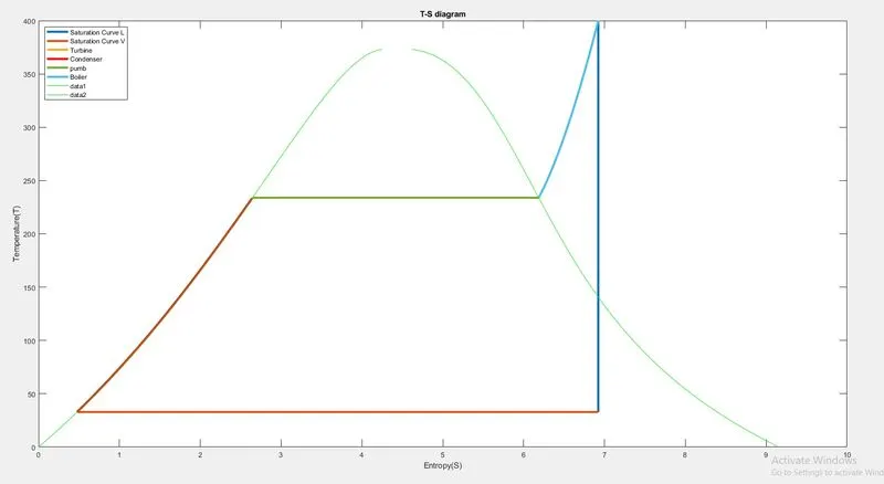
The above commands are used to plot the TS figure by using the calculated values. In this from state point 4 to 5 and state point 6 to the entropy values are given in array, beacuse the plot is curve for this state. So for having curve entropy values are defined in the array.
And the other commands are the calculated values to plot the TS diagram. In the figure xlabel, ylabel, title and legend command is used in order to have better understanding.
%Saturation curve for TS
t = linspace(0,373.15,500);
for i= 1:length(t)
    %Saturated liquid line
    sL(i) = XSteam('sL_T',t(i));
    sV(i) = XSteam('sV_T',t(i));

end

plot(sL,t,'g')
hold on
plot(sV,t,'g')
The above commands are used to plot saturated line for TS diagram. In here the maximum critical temperature is upto 373 so the range is given from 0 to 373 and 500 values is readed from this range to plot the saturated curve
%Plot the HS diagram

figure(2)

% 1 to 2
plot ([s1 s2],[h1 h2],'linewidth',3)
hold on

% 2 to 3
hc1 = linspace(h2,h3,1000);
pc3 = linspace(input_3,p3,1000);
for i=1:length(hc1)
    sc3(i) = XSteam('s_ph',pc3(i),hc1(i));
end
plot (sc3,hc1,'linewidth',3)

% 3 to 4
plot ([s3 s4],[h3 h4],'linewidth',3)

% 4 to 5
hc2 = linspace(h4,h5,1000);
pc4 = linspace(p4,p5,1000);
for i=1:length(hc2)
    sc4(i) = XSteam('s_ph',pc4(i),hc2(i));
end
plot (sc4,hc2,'linewidth',3)

% 5 to 6
hc3 = linspace(h5,h6,1000);
pc5 = linspace(p5,p6,1000);
for i=1:length(hc3)
    sc5(i) = XSteam('s_ph',pc5(i),hc3(i));
end
plot (sc5,hc3,'linewidth',3)

% 6 to 1
hc4 = linspace(h6,h1,1000);
pc6 = linspace(p6,input_1,1000);
for i=1:length(hc4)
    sc6(i) = XSteam('s_ph',pc6(i),hc4(i));
end
plot (sc6,hc4,'linewidth',3)
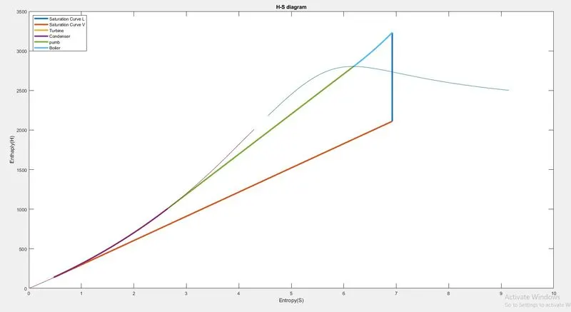
This commands are used to plot the HS diagram. For 1 to 2 and 3 to 4 values are given on the plot command, because the plot is a straight line. But for other the plot is a curve, so to get a curve the values are given in array. Within this array range the cuve is plotted for each state.
%Saturation curve for HS
 t2=linspace(0,input_2,1000);
 for j=1:length(t2)
     sl(j)=XSteam('sL_T',t2(j));
     sv(j)=XSteam('sV_T',t2(j));
     hl(j)=XSteam('hL_T',t2(j));
     hv(j)=XSteam('hV_T',t2(j));
end

plot(sl,hl)
hold on
plot(sv,hv)
legend('Saturation Curve L','Saturation Curve V','Turbine','Condenser','pumb','Boiler','location','northwest')
xlabel('Entropy(S)')
ylabel('Enthaply(H)')
title('H-S diagram')
The above commands are used to plot the HS saturated curve.
Results
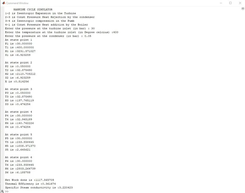
T-S plot
H-S plot