Project 2 - Rankine cycle Simulator

AIM

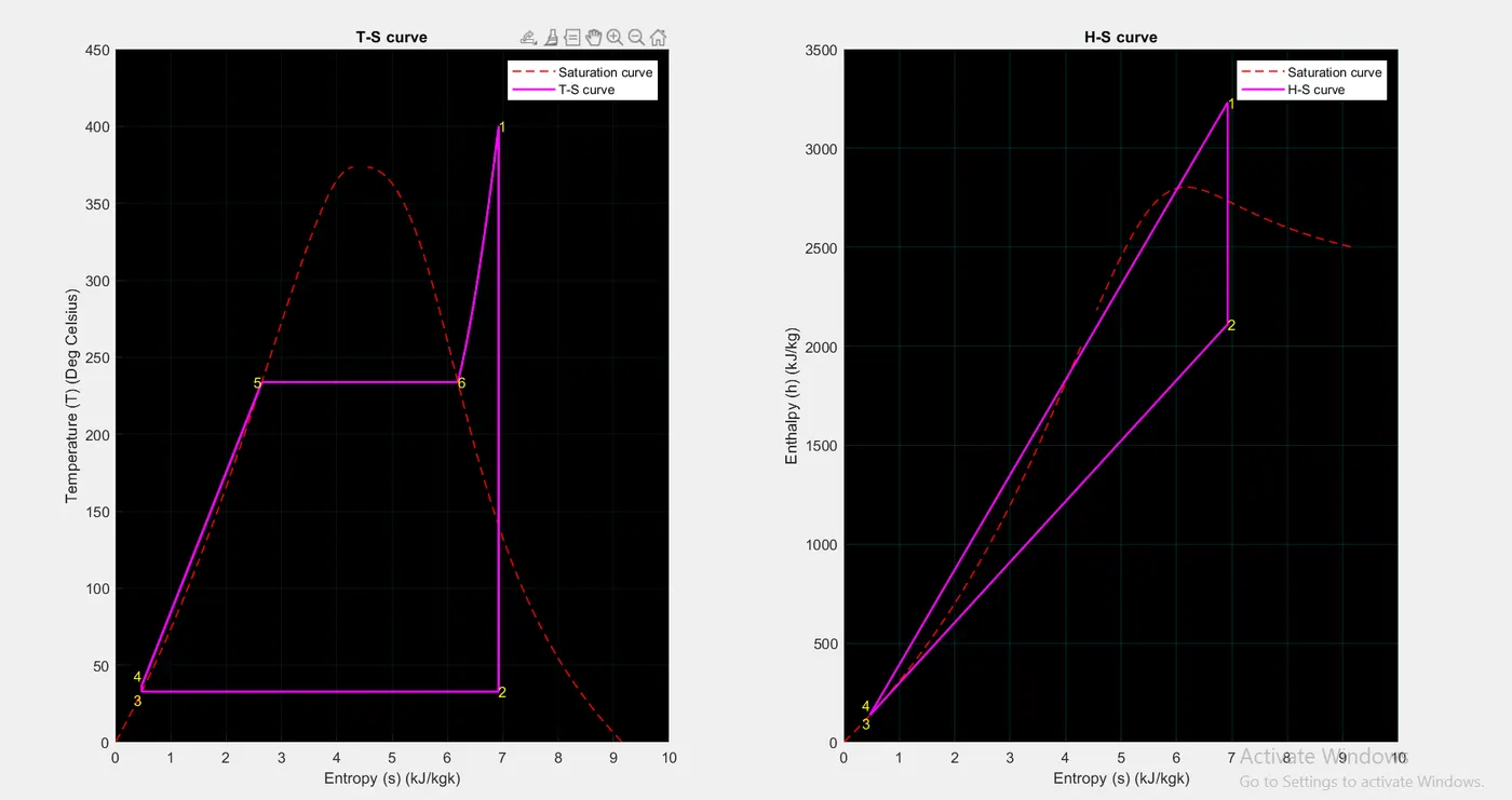
To create a Rankine Cycle Simulator using MATLAB and the code should calculate the state points of the Rankine Cycle based on the user defined inputs. And to plot the corresponding T-s and h-s plots for the given set of inputs. Title and axes labels are a must, while legends could be used if necessary.

OBJECTIVE

• To generate a code for Rankine cycle simulator for calclating the state points.
• To plot the graph between TS and HS diagram of Rankine cycle.

RANKINE CYCLE

Rankine cycle is the fundamental operating cycle of all thermal power plants where an operating fluid is continuously evaporated and condensed. It is the one of most common thermodynamic cycles, because in most of the places in the world the turbine is steam-driven.

In contrast to Carnot cycle, the Rankine cycle does not execute isothermal processes, because these must be performed very slowly. In an ideal Rankine cycle, the system executing the cycle undergoes a series of four processes: two isentropic (reversible adiabatic) processes alternated with two isobaric processes.

One of the major advantages of the Rankine cycle is that the compression process in the pump takes place on a liquid. By condensing the working steam to a liquid (inside a condenser) the pressure at the turbine outlet is lowered and the energy required by the feed pump consumes only 1% to 3% of the turbine output power and these factors contribute to a higher efficiency for the cycle.

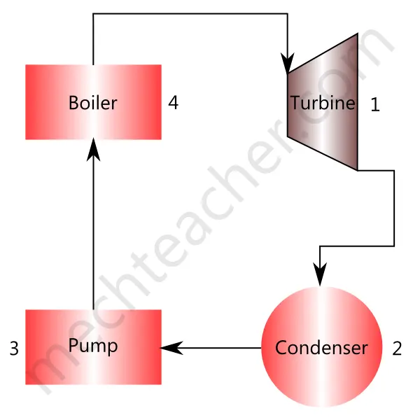
Process 1-2 : Isentropic Expansion in the Turbine.

Process 2-3 : Constant pressure heat rejection by the condenser.

Process 3-4 : Isentropic Compression in the Pump.

Process 4-1 : Constant pressure heat addition by the boiler.

Work done by the turbine is Wt.

Work done by the Pump is Wp.

Qin : Heat addition in the boiler.

Qout: Heat removal in the condenser.

Wnet : Net workdone is defined as the work from the trurbine is reduced from the work by the pump.

Nthermal : Thermal efficiency of the Rankine cycle.

PROGRAM DESCRIPTION

First of all the link for the standard Xsteam library to get the steam table data for water, is given.

Drive link of XSteam Library

It is used to calculate the points in between the state variables. The required inputs were given such as Turbine Inlet Pressure (P1) = 30 bars, Turbine Inlet temperature (T1) = 400° C, Turbine Outlet Pressure (P2) = 0.05 bars = Condenser Inlet Pressure.

1. An Output screen is given to obtain the command window as same as given. Inorder to obtain the same window Title and Four processes of the Rankine cycle were printed using fprintf command.
2. Then the input variables were assigned inorder to make it as a user defined inputs. That is user has to assign the values at the time of execution.
3. The Entropy and Enthalpy for the state variables 1 were get using the XSteam library.
4. Then the variables fo the state point 1 were printed in the command window using fprintf command.
5. Likewise the state points of 2,3,4 were find out using XSteam Library based on the user defined input values.
6. Here x is considered as dryness fraction.
7. In program we have given a if condition to calculate inlet temperature of condenser. If dryness fraction is less than 1, then T2 is taken as Saturation temperature for the related pressure P2. Else If dryness fraction is greater than 1, then temperature is calculated for related pressure and entropy.
8. Then after calculating all the state variables of all six state points. Other parameters were calculated and made printed on the output command window.
9. Graphs were plotted between Temperature and entropy and between Enthalpy and Entropy.

MATLAB CODE

%Title
fprintf('%50s\n\n',' RANKINE CYCLE SIMULATION')

%Processes of rankine cycle
fprintf('1-2 is Isentropic Expansion in the Turbine\n')
fprintf('2-3 is Const Pressure Heat Rejection by the Condenser\n')
fprintf('3-4 is Isentropic Compression in the Pump\n')
fprintf('4-1 is Const Pressure Heat Addition by the Boiler\n\n')

%Input parameters
p1 = input('Enter the Pressure at the Turbine Inlet (in bar):');
T1 = input('Enter the Temperature at the turbine inlet (in Degree celcius:');
p2 = input('Enter the Pressure at the Condenser (in bar):');

fprintf('\n%50s\n','RESULTS')

%State point 1
h1 = XSteam('h_pt',p1,T1);
s1 = XSteam('s_pt',p1,T1);

%To print the state point 1 values
fprintf('At State point 1 \n');
fprintf('P1 is : %4.2f Bar \n',p1);
fprintf('T1 is : %4.2f Deg Celsius \n',T1);
fprintf('H1 is : %4.2f kJ/kg \n',h1);
fprintf('S1 is : %4.2f kJ/kgk \n\n',s1);


%State point 2
s2 = s1;
sf2 = XSteam('sL_p',p2);
sg2 = XSteam('sV_p',p2);
hf2 = XSteam('hL_p',p2);
hg2 = XSteam('hV_p',p2);
x2 = ((s2-sf2)/(sg2-sf2));  %Dryness fraction
h2 = hf2+(x2*(hg2-hf2));

if (x2<1)
    T2 = XSteam('Tsat_p',p2);
else
    T2 = XSteam('T_ps',p2,s2);
end
    

%To print the state point 2 values
fprintf('At State point 2 \n');
fprintf('P2 is :%4.2f Bar \n',p2);
fprintf('T2 is : %4.2f Deg Celsius \n',T2);
fprintf('H2 is : %4.2f kJ/kg \n',h2);
fprintf('S2 is : %4.2f kJ/kgk \n',s2);
fprintf('X2 is : %4.2f \n\n',x2);


%State point 3
p3 = p2;
T3 = T2;
h3 = XSteam('hL_T',T3);
s3 = XSteam('sL_T',T3);

%To print the state point 3 values
fprintf('At State point 3 \n');
fprintf('P3 is : %4.2f Bar \n',p3);
fprintf('T3 is : %4.2f Deg Celsius \n',T3);
fprintf('H3 is : %4.2f kJ/kg \n',h3);
fprintf('S3 is : %4.2f kJ/kgk \n\n',s3);


%State point 4
p4 = p1;
s4 = s3;
h4 = XSteam('h_ps',p4,s4);
Cp4 = XSteam('Cp_ps',p4,s4);
Cv4 = XSteam('Cv_ps',p4,s4);
gamma = Cp4/Cv4;
g = (gamma-1)/gamma;
T4 = T3*((p4/p3)^g);

%To print the state point 4  values
fprintf('At State point 4 \n');
fprintf('P4 is : %4.2f Bar \n',p4);
fprintf('T4 is : %4.2f Deg Celsius \n',T4);
fprintf('H4 is : %4.2f kJ/kg \n',h4);
fprintf('S4 is : %4.2f kJ/kgk \n\n',s4);

%Turbine work
Wt = h1 - h2;
fprintf('Wt is : %4.2f kJ/kg \n',Wt);

%Pump work
Wp = h4 - h3;
fprintf('Wp is : %4.2f kJ/kg \n', Wp);

%Net work
Wnet = Wt - Wp;
fprintf('Wnet is : %4.2f kJ/kg \n',Wnet);

%To calculate Thermal efficiency
Qin = h1 - h4;
Qout = h2 - h3;
Ntherm = (Wnet/Qin)*100; %100 is multiplied to get the percentage value
fprintf('Ntherm is : %4.2f Percent \n',Ntherm);

%Specific Steam Consumption
SSC = (3600/(Wt-Wp)); %3600 is multiplied to convert it to kg/kWh from kg/kJ
fprintf('S.S.C is : %4.2f kg/kWh \n', SSC);


%State point 5
T5 = XSteam('Tsat_p',p1);
s5 = XSteam('sl_p',p1);
h5 = XSteam('hl_p',p1);


%State point 6
T6 = T5;
s6 = XSteam('sv_p',p1);
h6 = XSteam('hv_p',p1);


%Plotting Graphs
%T-S Diagram
subplot(1,2,1) 
Temperature_curve = linspace(0,T1,1000);    
for i = 1:length(Temperature_curve)
    s_l(i) = XSteam('sl_t',Temperature_curve(i));
    s_v(i) = XSteam('sv_t',Temperature_curve(i));
    
    h_l(i) = XSteam('hl_t',Temperature_curve(i));
    h_v(i) = XSteam('hv_t',Temperature_curve(i));
end

grid on
hold on

%To plot T-S Curve
plot([s_l,s_v],[Temperature_curve,Temperature_curve],'color','r','linestyle','--','linewidth',1);
axis([0 10 0 450])

Temperature = linspace(T5,T1,5000);
for i = 1:length(Temperature)
    Entropy(i) = XSteam('s_pt',p1,Temperature(i));
end
plot([s1 s2 s3 s4 s5 s6 Entropy],[T1 T2 T3 T4 T5 T6 Temperature],'color','m','linewidth',1.5);

%To mark the state points
text(s1,T1,'1','HorizontalAlignment','left','color','y')
text(s2,T2,'2','HorizontalAlignment','left','color','y')
text(s3,T3,'3','VerticalAlignment','top','HorizontalAlignment','right','color','y')
text(s4,T4,'4','VerticalAlignment','bottom','HorizontalAlignment','right','color','y')
text(s5,T5,'5','HorizontalAlignment','right','color','y')
text(s6,T6,'6','HorizontalAlignment','left','color','y')

%Labelling of Axes
xlabel('Entropy (s) (kJ/kgk)');
ylabel('Temperature (T) (Deg Celsius)');
legend('Saturation curve','T-S curve');
title('T-S curve');

%Setting background color for the plot
set(gca,'color',[0,0,0]);
ax = gca;
ax.GridColor = [0, .5, .5];
hold off


%H-S diagram
subplot(1,2,2)
hold on

%To plot the H-S curve
plot([s_l,s_v],[h_l,h_v],'color','r','linestyle','--','linewidth',1);

plot([s1 s2 s3 s4 s1],[h1 h2 h3 h4 h1],'color','m','linewidth',1.5);

%To mark the state points
text(s1,h1,'1','HorizontalAlignment','left','color','y')
text(s2,h2,'2','HorizontalAlignment','left','color','y')
text(s3,h3,'3','HorizontalAlignment','right','VerticalAlignment','top','color','y')
text(s4,h4,'4','HorizontalAlignment','right','VerticalAlignment','bottom','color','y')

%Labelling the Axes
xlabel('Entropy (s) (kJ/kgk)');
ylabel('Enthalpy (h) (kJ/kg)');
legend('Saturation curve','H-S curve');
title('H-S curve');

%To set background color for the plot
set(gca,'color',[0,0,0]);
ax = gca;
ax.GridColor = [0, 1, 1];
hold off
grid on

COMMAND WINDOW

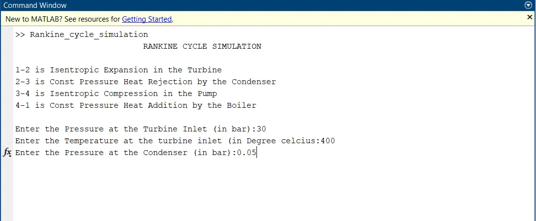
Getting inputs from the user.

OUTPUT WINDOW

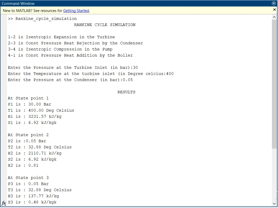
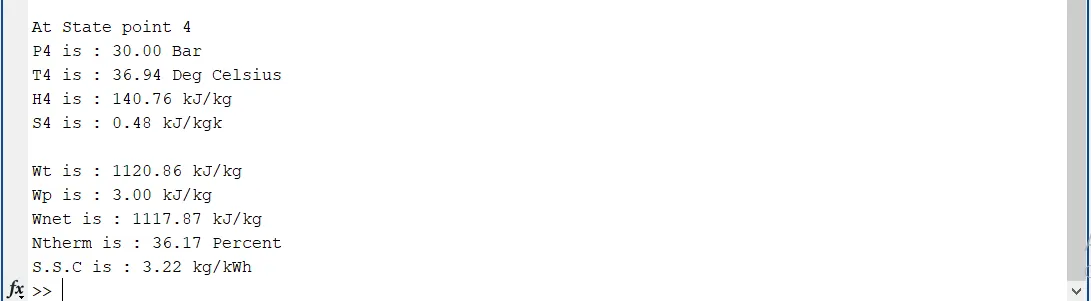
GRAPHS

ERRORS FACED

The errors faced were so simple in typing program like missings of semi-colons and wile plotting the graphs x and y values were mis-matched. These were rectified soon as error occured.

LEARNINGS

Where able to use previous learnt inbuilt commands in the graph this program. And learnt on rankine cycle simulation in matlab.

RESULTS AND CONCLUSION

A Rankine Cycle Simulator using MATLAB were created and Calculation of the state points of the Rankine Cycle were coded based on the user defined inputs. And the corresponding T-s and h-s plots for the given set of inputs were plotted. Title, axes and legends were used in needed area.