Project 2 - Rankine cycle Simulator
AIM:
Calculate the state points of the Rankine Cycle (any type of your choice) based on user inputs.
Objective:
- Create a Rankine Cycle Simulator using MATLAB.
- Calculate the state points of the Rankine Cycle (any type of your choice) based on user inputs.
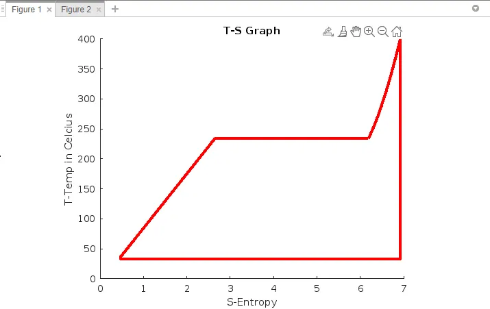
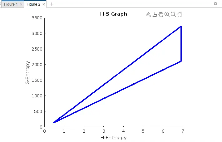
- Then, plot the corresponding T-s and h-s plots for the given set of inputs.
RANKINE CYCLE:
1-2: Isentropic Expansion in turbine.
2-3: constant pressure heat rejection at condenser.
3-4: Isentropic compression in pump.
4-1: constant pressure heat addition at boiler.
USED FORMULAS:
To calculate net work done and efficiency
wnet=wt−wp
ηth=(wnet\Qi)⋅100
where
wt=H1−H2
wp=H4−H3
Qi=H1−H4
To calculate the Specific Steam Consumption
S.S.C=3600/Wnet
To calculate the Back Work Ratio
B.W.R=(H1−H4/H2−H3)
CODING:
clear all
close all
clc
%inputs
%Turbine Inlet temperature T1= 400° C
%Turbine Inlet Pressure P1= 30 bars
%Turbine Outlet Pressure P2= 0.05 bars
% Condenser Inlet Pressure = 0.05 bars
R=8.314;
% at state point:1
p1=30;
p2=0.05;
t1=400;
calling the variables from Xsteam file.
% 1-2: isentropic compression
S1 = XSteam('s_pT',p1,t1);
H1 = XSteam('h_pT',p1,t1);
% at point 2
S2=S1;
sf2 = XSteam('sL_p',p2);
sg2 = XSteam('sV_p',p2);
hf2 = XSteam('hL_p',p2);
hg2 = XSteam('hV_p',p2);
t2 = XSteam ('Tsat_p',p2);
x2 = ((S2-sf2)/(sg2-sf2));
H2 = hf2+(x2*(hg2-hf2));
% At State Point 3
p3 = p2;
t3 = XSteam('Tsat_p',p3);
S3 = XSteam('sL_p',p3);
H3 = XSteam('hL_p',p3);
% To calculate Gamma
cp = XSteam('cpL_p',p3);
cv = XSteam('cvL_p',p3);
gamma = (cp/cv);
% At State Point 4
p4 = p1;
S4 = S3;
H4 = XSteam('h_ps',p4,S4);
t4 = t3*((p4/p3)^((gamma-1)/gamma));
% Calculating work done
wt = H1 - H2;
wp = H4 - H3;
wnet = wt-wp;
qin = H1 - H4;
qout = H2 - H3;
n = wnet/qin;
n_percent = n*100;
SSC = 3600/wnet;
BWR = qin/qout;
% At State Points 5 and 6
t5 = XSteam('Tsat_p',p1);
t6 = t5;
S5 = XSteam('sL_p',p1);
S6 = XSteam('sV_p',p1);
H5 = XSteam('hL_p',p1);
H6 = XSteam('hV_p',p1);
% Plotting The Required Graphs
% T-S Graph
figure(1)
T = linspace(t5,t1,500);
for i = 1:length(T)
S(i) = XSteam('s_pt',p1,T(i));
end
hold on
plot([S1 S2 S3 S4 S5 S6 S],[t1 t2 t3 t4 t5 t6 T],'linewidth',3,'color','r')
xlabel('S-Entropy');
ylabel('T-Temp in Celcius');
title('T-S Graph');
% H-S Graph
figure(2)
hold on
plot([S1 S2 S3 S4 S1],[H1 H2 H3 H4 H1],'linewidth',3,'color','b')
xlabel('H-Enthalpy');
ylabel('S-Entropy');
title('H-S Graph');
f1=fopen('rank.txt','w') -----used to crate txt file
fprintf(f1,'RANKINE CYCLE SIMULATOR \n');
fprintf(f1,'RESULTS\n');
fprintf(f1,'AT POINT 1:\n');
fprintf(f1,'P1 is:%f\n',p1);
fprintf(f1,'T1 is:%f\n',t1);
fprintf(f1,'S1 is:%f\n',S1);
fprintf(f1,'H1 is:%f\n',H1);
fprintf(f1,'AT POINT 2:\n');
fprintf(f1,'P2 is:%f\n',p2);
fprintf(f1,'T2 is:%f\n',t2);
fprintf(f1,'S2 is:%f\n',S2);
fprintf(f1,'H2 is:%f\n',H2);
fprintf(f1,'x2 is:%f\n',x2);
fprintf(f1,'AT POINT 3:\n');
fprintf(f1,'P3 is:%f\n',p3);
fprintf(f1,'T3 is:%f\n',t3);
fprintf(f1,'S3 is:%f\n',S3);
fprintf(f1,'H3 is:%f\n',H3);
fprintf(f1,'AT POINT 4:\n');
fprintf(f1,'P4 is:%f\n',p4);
fprintf(f1,'T4 is:%f\n',t4);
fprintf(f1,'S4 is:%f\n',S4);
fprintf(f1,'H4 is:%f\n',H4);
fprintf(f1,'Wt is :%f \n',wt);
fprintf(f1,'Wp is : %f\n',wp);
fprintf(f1,'Wnet is:%f\n ',wnet);
fprintf(f1,'Ntherm is:%f\n',n_percent);
fprintf(f1,'SSC is:%f \n',SSC);
fprintf(f1,'BWR is:%f \n',BWR);
fclose(f1);
out put:
links: