Project 2 - Rankine cycle Simulator
Project 2 - Rankine cycle Simulator:
Aim:
- Calculate state points in the Rankine Cycle based on user inputs.
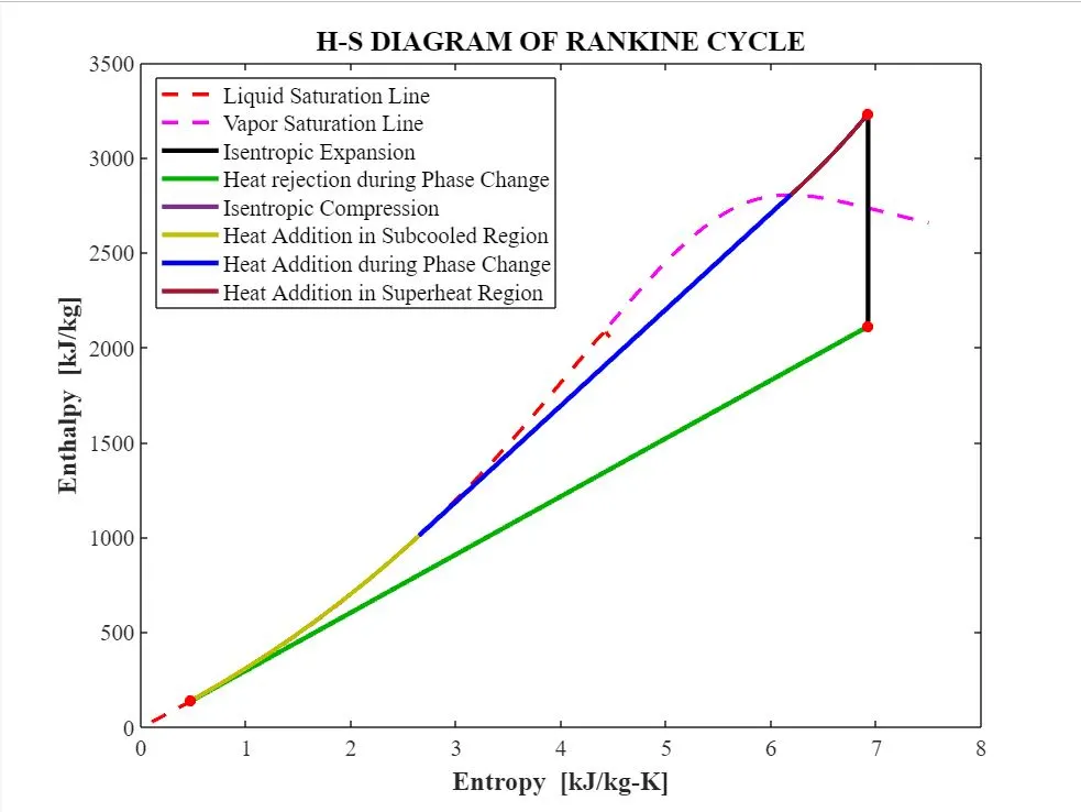
- Plot corresponding T-s (Temperature-Entropy) and h-s (Enthalpy-Entropy) diagrams.
Introduction to Rankine Cycle:
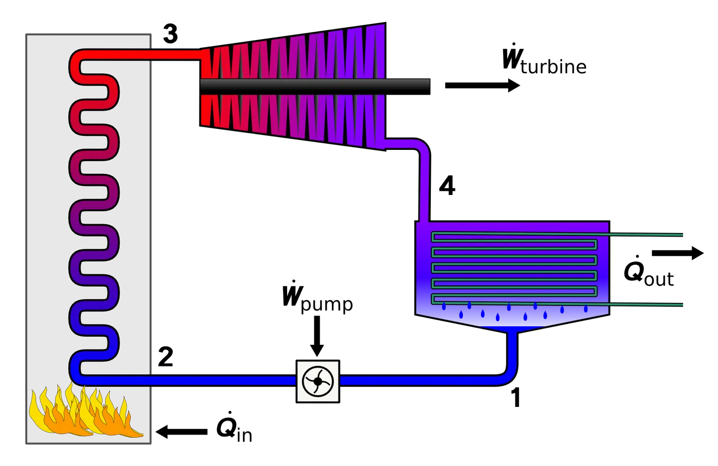
The Rankine Cycle is a fundamental process used in power plants to convert heat into mechanical energy, eventually generating electricity. It involves four main components: Turbine, Condenser, Pump, and Boiler.
-
Turbine (Process: 1-2):
- Isentropic Expansion: Superheated vapor expands in the turbine, producing work (W_T). The exit state can be superheated, saturated vapor, or liquid-vapor mix.
��=�⋅(ℎ1−ℎ2)
-
Condenser (Process: 2-3):
- Isobaric Heat Rejection: The vapor-liquid mixture is condensed at constant low pressure, extracting heat (Q_add).
����=�⋅(ℎ2−ℎ3
-
Pump (Process: 3-4):
- Isentropic Compression: The condensate is raised isentropically in the feed pump with relatively small pump work
��=�⋅(ℎ4
-
Boiler (Process: 4-1):
- Isobaric Heat Transfer: High-pressure liquid enters the boiler, gets heated, and undergoes phase change until it becomes superheated steam.
����=�⋅(ℎ1
Specific steam consumption (SSC) is the amount of steam required to produce 1 kilowatt (kW) of net work output in a steam turbine power plant.���=3600��−��
PV and TS Diagram:
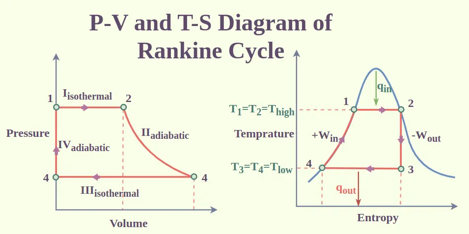
Rankine Cycle - P-v Diagram:
1.Isentropic Expansion (Process 1-2):
- The superheated vapor expands isentropically in the turbine (Process 1-2).
- This process is represented by an upward-sloping curve on the P-v diagram.
- The turbine work is done during this phase.
2.Isobaric Heat Rejection (Process 2-3):
- The vapor-liquid mixture leaves the turbine and is condensed at constant low pressure in the condenser (Process 2-3).
- This phase is represented by a horizontal line on the P-v diagram.
- Heat is rejected to the cooling medium, causing the vapor to condense.
3.Isentropic Compression (Process 3-4):
- The condensate is isentropically compressed in the feed pump (Process 3-4).
- On the P-v diagram, this is represented by an upward-sloping curve.
- Pump work is done to increase the pressure.
4.Isobaric Heat Addition (Process 4-1):
- High-pressure liquid enters the boiler, gets heated, and undergoes phase change until it becomes superheated steam (Process 4-1).
- The P-v diagram shows a curve representing heating at constant pressure.
Rankine Cycle - T-s Diagram:
1.Isentropic Expansion (Process 1-2):
- Superheated vapor expands isentropically in the turbine.
- On the T-s diagram, this process is represented by a vertical line.
2.Isobaric Heat Rejection (Process 2-3):
- Vapor-liquid mixture is condensed at constant low pressure in the condenser.
- This phase is represented by a horizontal line on the T-s diagram.
3.Isentropic Compression (Process 3-4):
- Condensate is isentropically compressed in the pump.
- On the T-s diagram, this is represented by another vertical line.
4.Isobaric Heat Addition (Process 4-1):
- High-pressure liquid enters the boiler and undergoes heating until it becomes superheated steam.
- This process is represented by a curve at constant pressure on the T-s diagram.
Code for Rankine cycle simulator:
% Rankine cycle simulator
clear all
close all
clc
fprintf('RANKINE CYCLE SIMULATOR\n')
fprintf('Process 1-2: Isentropic Expansion in Turbine\n')
fprintf('Process 2-3: Constant Presssure Heat Rejection in Condenser\n')
fprintf('Process 3-4: Isentropic Compression in Pump\n')
fprintf('Process 4-1: Constant Presssure Heat Addition in Boiler\n')
% STATE 1: TURBINE INLET or BOILER OUTLET
p1 = input('Enter Pressure at Turbine Inlet in bar : ');
T1 = input('Enter Temperature at Turbine Inlet in degree Celcius : ');
% STATE 2: TURBINE OUTLET or CONDENSER INLET
p2 = input('Enter Pressure at Condenser Inlet in bar : ');
% CALCULATIONS
% STATE 1: TURBINE INLET or BOILER OUTLET
h1 = XSteam('h_pT',p1,T1);
s1 = XSteam('s_pT',p1,T1);
% STATE 2: TURBINE OUTLET or CONDENSER INLET
s2 = s1;
sf2 = XSteam('sL_p',p2);
sg2 = XSteam('sV_p',p2);
x2 = (s2-sf2)/(sg2-sf2);
hf2 = XSteam('hL_p',p2);
hg2 = XSteam('hV_p',p2);
if x2 <= 1 % IF POINT 2 IS IN LIQUID-VAPOR MIXTUE REGION OR SATURATED VAPOR STATE
h2 = hf2 + x2*(hg2 - hf2);
T2 = XSteam('T_ph',p2,h2);
else % IF POINT 2 IS IN SUPERHEATED REGION
Tsat_p2 = XSteam('Tsat_p',p2);
T2 = XSteam('T_ps',p2,s2);
CpV = XSteam('Cp_pT',p2,T2);
h2 = hg2 + CpV*(T2 - Tsat_p2);
end
% STATE 3: CONDENSER OUTLET or PUMP INLET
p3 = p2;
h3 = XSteam('hL_p',p3);
s3 = XSteam('sL_p',p3);
v3 = XSteam('vL_p',p3);
T3 = XSteam('Tsat_p',p3);
% STATE 4: PUMP OUTLET or BOILER INLET
p4 = p1;
s4 = s3;
h4 = XSteam('h_ps',p4,s4);
T4 = XSteam('T_ph',p4,h4);
% PROPERTIES AT SATURATION LIQUID STATE ON BOILER PRESSURE
h4_SatL_p4 = XSteam('hL_p',p4);
s4_SatL_p4 = XSteam('sL_p',p4);
% PROPERTIES AT SATURATION VAPOUR STATE ON BOILER PRESSURE
h4_SatV_p4 = XSteam('hV_p',p4);
s4_SatV_p4 = XSteam('sV_p',p4);
% SATURATION TEMPERATURE ON BOILER PRESSURE
Tsat_p4 = XSteam('Tsat_p',p4);
% TO PLOT T-S, H-S DIAGRAMS IN SUPERHEATED REGION OF BOILER, CALCULATION OF T & H at INTERMEDIATE POINTS
Superheat_entropy_range = linspace(s4_SatV_p4,s1,10000);
for i=1:length(Superheat_entropy_range)
Superheat_enthalpy_range(i) = XSteam('h_ps',p1,Superheat_entropy_range(i));
Superheat_Temp_range(i) = XSteam('T_ps',p1,Superheat_entropy_range(i));
end
% TO PLOT T-S, H-S DIAGRAMS IN SUBCOOLED REGION OF BOILER, CALCULATION OF T & H at INTERMEDIATE POINTS
Subcool_entropy_range = linspace(s4,s4_SatL_p4,10000);
for i=1:length(Subcool_entropy_range)
Subcool_enthalpy_range(i) = XSteam('h_ps',p1,Subcool_entropy_range(i));
Subcool_Temp_range(i) = XSteam('T_ps',p1,Subcool_entropy_range(i));
end
% FINDING SATURATION TEMPERATURES CORRESPONDING TO ENTROPY (HELPFUL TO PLOT SATURATION LINE ON T-S DIAGRAM)
S_min = 0.1;
S_max = 7.5;
S = linspace(S_min,S_max,1000);
for i=1:length(S)
Tsat(i) = XSteam('Tsat_s',S(i));
end
% FINDING ENTROPY AT CRITICAL POINT USING CRITICAL PRESSURE AND CRITICAL TEMPERATURE OF WATER
% CRITICAL TEMPERATURE OF WATER : 373.946 degree Celcius
% CRITICAL PRESSURE OF WATER : 220.635 bar
S_Critical = XSteam('s_pT',220.635,373.946);
% FINDING SATURATION ENTHALPIES USING ENTROPY AND SATURATION PRESSURE (HELPFUL TO PLOT SATURATION LINE ON H-S DIAGRAM)
% LIQUID STATE SATURATION ENTHAPIES i.e, BEFORE CRITICAL POINT OF WATER
S_SatL = linspace(S_min,S_Critical,1000);
for i=1:length(S_SatL)
PsatL(i) = XSteam('Psat_s',S_SatL(i));
HSatL(i) = XSteam('hL_p',PsatL(i));
end
% FINDING SATURATION ENTHALPIES USING ENTROPY AND SATURATION PRESSURE (HELPFUL TO PLOT SATURATION LINE ON H-S DIAGRAM)
% GASEOUS STATE SATURATION ENTHAPIES i.e, AFTER CRITICAL POINT OF WATER
S_SatV = linspace(S_Critical,S_max,1000);
for i=1:length(S_SatV)
PsatV(i) = XSteam('Psat_s',S_SatV(i));
HSatV(i) = XSteam('hV_p',PsatV(i));
end
% PLOTTING T-S DIAGRAM
figure('DefaultAxesFontSize',12)
% SATURATION LINE
plot(S,Tsat,'--','linewidth',2,'color','r')
hold on
% PROCESS 1-2: ISENTROPIC PROCESS (VERTICAL STRAIGHT LINE IN T-S DIAGRAM)
plot([s1 s2],[T1 T2],'linewidth',2.5,'color','k')
hold on
% PROCESS 2-3: CONSTANT PRESSURE PROCESS IN WHICH PHASE CHANGE OCCURS FROM SATURATED OR SUPERHEATED VAPOR OR LIQUID-VAPOR MIX TO SATURATED LIQUID
if x2 <= 1
% IT WILL BE A HORIZONTAL STRAIGHT LINE IN T-S DIAGRAM
plot([s2 s3],[T2 T3],'linewidth',2.5,'color',[0, 0.7, 0])
hold on
else
% TO PLOT T-S, H-S DIAGRAMS IN SUPERHEATED REGION, CALCULATION OF T & H at INTERMEDIATE POINTS
Superheat_cond_entropy = linspace(s2,sg2,1000);
for i=1:length(Superheat_cond_entropy)
Superheat_cond_enthalpy(i) = XSteam('h_ps',p2,Superheat_cond_entropy(i));
Superheat_cond_Temp(i) = XSteam('T_ps',p2,Superheat_cond_entropy(i));
end
plot(Superheat_cond_entropy,Superheat_cond_Temp,'linewidth',2.5,'color',[0, 0.8, 0.8])
% IT WILL BE A HORIZONTAL STRAIGHT LINE IN T-S DIAGRAM
plot([sg2 s3],[Tsat_p2 T3],'linewidth',2.5,'color',[0, 0.7, 0])
end
% PROCESS 3-4: ISENTROPIC PROCESS (VERTICAL STRAIGHT LINE IN T-S DIAGRAM)
plot([s3 s4],[T3 T4],'linewidth',2.5,'color','m')
legend
hold on
% PROCESS 4-1: CONSTANT PRESSURE PROCESS
% IT CONTAINS 3 REGIONS
% REGION 1: SUBCOOLED REGION :: IN LIQUID REGION (CURVE ALONG CONSTANT PRESSURE LINES IN T-S DIAGRAM)
plot(Subcool_entropy_range,Subcool_Temp_range,'linewidth',2.5,'color',[0.75, 0.75, 0])
hold on
% REGION 2: LIQUID-VAPOR REGION :: PHASE CHANGE OCCURS FROM LIQUID TO GAS (HORIZONTAL STRAIGHT LINE IN T-S DIAGRAM)
plot([s4_SatL_p4 s4_SatV_p4],[Tsat_p4 Tsat_p4],'linewidth',2.5,'color','b')
hold on
% REGION 3: SUPERHEAT REGION :: IN GASEOUS STATE (CURVE ALONG CONSTANT PRESSURE LINES IN T-S DIAGRAM)
plot(Superheat_entropy_range,Superheat_Temp_range,'linewidth',2.5,'color',[0.6350, 0.0780, 0.1840])
% MARKING ALL STATE POINTS
plot(s1, T1, 'o', 'MarkerSize', 4, 'MarkerfaceColor', 'r', 'MarkerEdgeColor', 'r', 'linewidth', 2);
plot(s2, T2, 'o', 'MarkerSize', 4, 'MarkerfaceColor', 'r', 'MarkerEdgeColor', 'r', 'linewidth', 2);
plot(s3, T3, 'o', 'MarkerSize', 4, 'MarkerfaceColor', 'r', 'MarkerEdgeColor', 'r', 'linewidth', 2);
plot(s4, T4, 'o', 'MarkerSize', 4, 'MarkerfaceColor', 'r', 'MarkerEdgeColor', 'r', 'linewidth', 2);
xlabel('Entropy [kJ/kg-K]', 'FontSize', 14,'FontWeight','bold');
ylabel('Temperature [^0C]', 'FontSize', 14,'FontWeight','bold');
title('T-S DIAGRAM OF RANKINE CYCLE', 'FontSize', 15);
% SETTING ALL THE FONTS IN FIGURE TO TIMES NEW ROMAN
if x2<=1
legend('Saturation Line','Isentropic Expansion','Heat rejection during Phase Change','Isentropic Compression','Heat Addition in Subcooled Region','Heat Addition during Phase Change','Heat Addition in Superheat Region', 'location', 'NorthWest','FontSize',12);
else
legend('Saturation Line','Isentropic Expansion','Heat Rejection during Superheat Region','Heat Rejection during Phase Change','Isentropic Compression','Heat Addition in Subcooled Region','Heat Addition during Phase Change','Heat Addition in Superheat Region', 'location', 'NorthWest','FontSize',12);
end
set(findall(gcf,'-property','FontName'),'FontName','Times New Roman')
% PLOTTING H-S DIAGRAM
figure('DefaultAxesFontSize',12)
% SATURATION LINE BEFORE CRITICAL POINT i.e LIQUID SATURATION LINE
plot(S_SatL,HSatL,'--','linewidth',2,'color','r')
hold on
% SATURATION LINE AFTER CRITICAL POINT i.e VAPOR SATURATION LINE
plot(S_SatV,HSatV,'--','linewidth',2,'color','m')
hold on
% PROCESS 1-2: ISENTROPIC PROCESS (VERTICAL STRAIGHT LINE IN H-S DIAGRAM)
plot([s1 s2],[h1 h2],'linewidth',2.5,'color','k')
hold on
% PROCESS 2-3: CONSTANT PRESSURE PROCESS IN WHICH PHASE CHANGE OCCURS FROM SATURATED OR SUPERHEATED VAPOR OR LIQUID-VAPOR MIX TO SATURATED LIQUID
if x2 <= 1
% IT WILL BE A STRAIGHT LINE IN H-S DIAGRAM
plot([s2 s3],[h2 h3],'linewidth',2.5,'color',[0, 0.7, 0])
else
plot(Superheat_cond_entropy,Superheat_cond_enthalpy,'linewidth',2.5,'color',[0, 0.8, 0.8])
% IT WILL BE A STRAIGHT LINE IN H-S DIAGRAM
plot([sg2 s3],[hg2 h3],'linewidth',2.5,'color',[0, 0.7, 0])
end
hold on
% PROCESS 3-4: ISENTROPIC PROCESS (VERTICAL STRAIGHT LINE IN H-S DIAGRAM)
plot([s3 s4],[h3 h4],'linewidth',2.5,'color',[0.4940, 0.1840, 0.5560])
hold on
% PROCESS 4-1: CONSTANT PRESSURE PROCESS
% IT CONTAINS 3 REGIONS
% REGION 1: SUBCOOLED REGION :: IN LIQUID REGION (CURVE ALONG CONSTANT PRESSURE LINES IN H-S DIAGRAM)
plot(Subcool_entropy_range,Subcool_enthalpy_range,'linewidth',2.5,'color',[0.75, 0.75, 0])
hold on
% REGION 2: LIQUID-VAPOR REGION :: PHASE CHANGE OCCURS FROM LIQUID TO GAS (STRAIGHT LINE IN H-S DIAGRAM)
plot([s4_SatL_p4 s4_SatV_p4],[h4_SatL_p4 h4_SatV_p4],'linewidth',2.5,'color','b')
hold on
% REGION 3: SUPERHEAT REGION :: IN GASEOUS STATE (CURVE ALONG CONSTANT PRESSURE LINES IN H-S DIAGRAM)
plot(Superheat_entropy_range,Superheat_enthalpy_range,'linewidth',2.5,'color',[0.6350, 0.0780, 0.1840])
xlabel('Entropy [kJ/kg-K]', 'FontSize', 14,'FontWeight','bold');
ylabel('Enthalpy [kJ/kg]', 'FontSize', 14,'FontWeight','bold');
title('H-S DIAGRAM OF RANKINE CYCLE', 'FontSize', 15);
% MARKING ALL STATE POINTS
plot(s1, h1, 'o', 'MarkerSize', 4, 'MarkerfaceColor', 'r', 'MarkerEdgeColor', 'r', 'linewidth', 2);
plot(s2, h2, 'o', 'MarkerSize', 4, 'MarkerfaceColor', 'r', 'MarkerEdgeColor', 'r', 'linewidth', 2);
plot(s3, h3, 'o', 'MarkerSize', 4, 'MarkerfaceColor', 'r', 'MarkerEdgeColor', 'r', 'linewidth', 2);
plot(s4, h4, 'o', 'MarkerSize', 4, 'MarkerfaceColor', 'r', 'MarkerEdgeColor', 'r', 'linewidth', 2);
if x2<=1
legend('Liquid Saturation Line','Vapor Saturation Line','Isentropic Expansion','Heat rejection during Phase Change','Isentropic Compression','Heat Addition in Subcooled Region','Heat Addition during Phase Change','Heat Addition in Superheat Region', 'location', 'NorthWest','FontSize',12);
else
legend('Liquid Saturation Line','Vapor Saturation Line','Isentropic Expansion','Heat Rejection during Superheat Region','Heat Rejection during Phase Change','Isentropic Compression','Heat Addition in Subcooled Region','Heat Addition during Phase Change','Heat Addition in Superheat Region', 'location', 'NorthWest','FontSize',12);
end
% SETTING ALL THE FONTS IN FIGURE TO TIMES NEW ROMAN
set(findall(gcf,'-property','FontName'),'FontName','Times New Roman')
% WORK PRODUCED BY TURBINE
Turbine_Work = h1 - h2;
% WORK CONSUMED BY PUMP
Pump_Work = h4 - h3;
% NET WORK PRODUCED IN RANKINE CYCLE
Net_Work = Turbine_Work - Pump_Work;
% HEAT INPUT IN BOILER
Q_In = h1 - h4;
% HEAT REJECTED IN CONDENSER
Q_Out = h2 - h3;
% EFFICIENCY OF RANKINE CYCLE
Thermal_Efficiency = (1 - (Q_Out/Q_In))*100;
% SPECIFIC STEAM CONSUMPTION
SSC = 3600/Net_Work;
% BACK WORK RATIO IN RANKINE CYCLE
Back_Work_Ratio = Pump_Work/Turbine_Work;
fprintf('RESULTS \n')
fprintf(' STATE POINT 1 \n')
fprintf('P1 = %4.3f bar\n',p1);
fprintf('T1 = %4.3f deg Celcius\n',T1);
fprintf('H1 = %4.3f kJ/kg\n',h1);
fprintf('S1 = %4.3f kJ/kg-K\n',s1);
fprintf(' STATE POINT 2 \n')
fprintf('P2 = %4.3f bar\n',p2);
fprintf('T2 = %4.3f deg Celcius\n',T2);
fprintf('H2 = %4.3f kJ/kg\n',h2);
fprintf('S2 = %4.3f kJ/kg-K\n',s2);
if x2 <= 1
fprintf('X2 = %4.3f\n',x2);
else
fprintf('STATE POINT 2 IS IN SUPERHEATED REGION\n');
end
fprintf(' STATE POINT 3 \n')
fprintf('P3 = %4.3f bar\n',p3);
fprintf('T3 = %4.3f deg Celcius\n',T3);
fprintf('H3 = %4.3f kJ/kg\n',h3);
fprintf('S3 = %4.3f kJ/kg-K\n',s3);
fprintf(' STATE POINT 4 \n')
fprintf('P4 = %4.3f bar\n',p4);
fprintf('T4 = %4.3f deg Celcius\n',T4);
fprintf('H4 = %4.3f kJ/kg\n',h4);
fprintf('S4 = %4.3f kJ/kg-K\n',s4);
fprintf('Turbine Work= %4.3f kJ/kg\n',Turbine_Work);
fprintf('Pump Work= %4.3f kJ/kg\n',Pump_Work);
fprintf('Net Work= %4.3f kJ/kg\n',Net_Work);
fprintf('Back Work Ratio = %4.6f\n',Back_Work_Ratio);
fprintf('Heat Input= %4.3f kJ/kg\n',Q_In);
fprintf('Heat Rejected= %4.3f kJ/kg\n',Q_Out);
fprintf('Therm_Eff= %4.3f Percent\n',Thermal_Efficiency);
fprintf('S.S.C= %4.3f kg/kWh\n',SSC);
User Input:
- The program starts by asking the user to input certain values:
- Pressure and temperature at the turbine inlet (where steam enters the turbine).
- Pressure at the condenser inlet (where steam enters the condenser).
- Pressure at the condenser outlet (where steam exists the condenser).
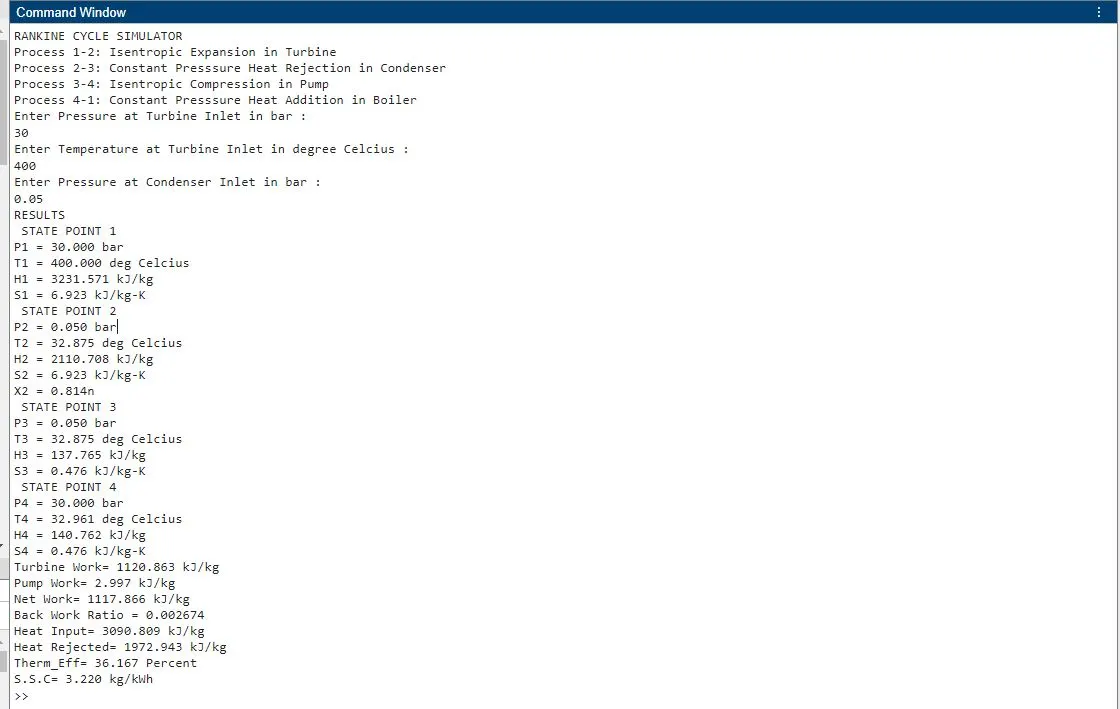
- Here given inputs are,
- Turbine Inlet temperature = 400° C
- Turbine Inlet Pressure = 30 bars
- Turbine Outlet Pressure = 0.05 bars = Condenser Inlet Pressure
Calculations:
- The code uses the XSteam library to calculate thermodynamic properties of water and steam at different states of the Rankine cycle (represented by points 1 to 4).
- It determines properties like enthalpy, entropy, temperature, and dryness fraction.
Plotting Diagrams:
The program then plots two diagrams:
- T-s (Temperature-Entropy) diagram, which shows the cycle on a graph with temperature and entropy as axes.
- H-s (Enthalpy-Entropy) diagram, which is another way to represent the same cycle using enthalpy and entropy.
Results and Outputs:
- The code calculates and prints various results of the Rankine cycle, such as turbine work, pump work, net work, back work ratio, heat input, heat rejection, thermal efficiency, specific steam consumption, etc.
Visualization:
- The T-s and H-s diagrams are displayed with marked points representing different states of the Rankine cycle.
Explanation of States:
- Information about each state (1 to 4) of the cycle is printed, including pressure, temperature, enthalpy, and entropy.
Output:
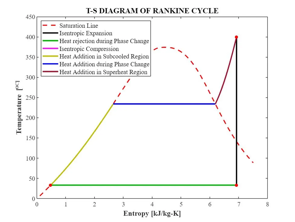
Output at comment box: