Project 2 - Rankine cycle Simulator
AIM: TO SIMULATE THE RANKINE CYCLE USING MATLAB.Understanding the concept of Rankine cycle by referring the standard thermal engineering text book.
PROCEDURE:
The link for the standard Xsteam library to get the steam table data for water, is given below. It must be used to calculate the points in between the state variables.
CODE:
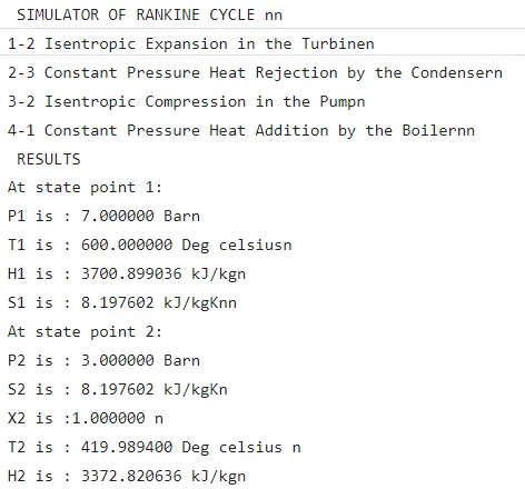
fprintf(' SIMULATOR OF RANKINE CYCLE nn')
fprintf('1-2 Isentropic Expansion in the Turbinen')
fprintf('2-3 Constant Pressure Heat Rejection by the Condensern')
fprintf('3-2 Isentropic Compression in the Pumpn')
fprintf('4-1 Constant Pressure Heat Addition by the Boilernn')
%inputs
P1 = input('Enter the Pressure at the Turbine Inlet (in bar): ');
T1 = input('Enter the Temperature at the Turbine inlet (in Degree celsius): ');
P2 = input('Enter the Pressure at the Condenser (in bar): ');
disp(' RESULTS')
%getting Cp and cv values from Xsteam
%Cp and Cv assumed to not change with temperature to make problem simple
% for vapur
high_cpV= XSteam('CpV_p', P1);
low_cpV=XSteam('CpV_p', P2);
high_cvV=XSteam('CvV_p', P1);
low_cvV=XSteam('CvV_p', P2);
% for liquid
high_cpL= XSteam('CpL_p', P1);
low_cpL=XSteam('CpL_p', P2);
high_cvL=XSteam('CvL_p', P1);
low_cvL=XSteam('CvL_p', P2);
%Getting important parameters from Xsteam
%for high pressure
T1s = XSteam('Tsat_p', P1);
S1g = XSteam('sV_p', P1);
S1f = XSteam('SL_p', P1);
S1fg = S1g - S1f;
H1f = XSteam('hL_p', P1);
H1g = XSteam('hV_p', P1);
H1fg = H1g - H1f;
%for low pressure
S2g = XSteam('sV_p', P2);
S2f = XSteam('SL_p', P2);
S2fg = S2g - S2f;
T2s = XSteam('Tsat_p', P2);
H2f = XSteam('hL_p', P2);
H2g = XSteam('hV_p', P2);
H2fg = H2g - H2f;
%% State point 1
disp('At state point 1:')
fprintf('P1 is : %f Barn', P1)
fprintf('T1 is : %f Deg celsiusn', T1)
H1 = XSteam('h_pt', P1, T1);
fprintf('H1 is : %f kJ/kgn', H1)
S1 = XSteam('s_pt', P1, T1);
fprintf('S1 is : %f kJ/kgKnn', S1)
%% State point 2
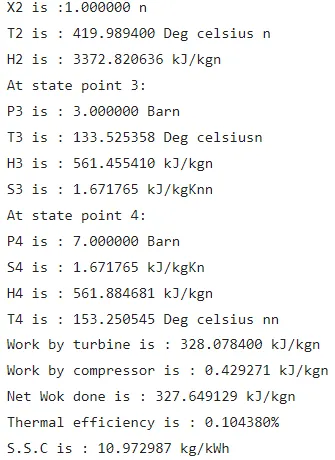
disp('At state point 2:')
fprintf('P2 is : %f Barn', P2) %P2 input already taken
S2 = S1;
fprintf('S2 is : %f kJ/kgKn', S2)
%predicting location of point 2 in T-s
if(S2<=S2g)
X2 = (S2 - S2f) / (S2fg); % Dryness Fraction at state point 2
else
X2=1;
end
fprintf('X2 is :%f n', X2)
%calculating T2 for superheat or wet or dry wherever it lies
if(X2<1)
T2=T2s;
else
%t2 cal by s2=s2g+low_cpV*(log(T2/T2s))
T2=(T2s+273.15)*exp((S2-S2g)/low_cpV) ; %2 in superheated region
T2=T2-273.15;
end
fprintf('T2 is : %f Deg celsius n', T2)
if(X2<1)
H2 = H2f + X2 * H2fg;
else
H2=H2g+ low_cpV*(T2-T2s);
end
fprintf('H2 is : %f kJ/kgn', H2)
%% State point 3
%Assuming no subcooling in condensor
disp('At state point 3:')
P3 = P2;
fprintf('P3 is : %f Barn', P3)
V3 = XSteam('vL_p', P3);
T3 = T2s; %no subcooling assumed
fprintf('T3 is : %f Deg celsiusn', T3)
H3 =H2f;
fprintf('H3 is : %f kJ/kgn', H3)
S3 =S2f;
fprintf('S3 is : %f kJ/kgKnn', S3)
%% State point 4
disp('At state point 4:')
P4 = P1;
fprintf('P4 is : %f Barn', P4)
S4 = S3;
fprintf('S4 is : %f kJ/kgKn', S4)
Wp = V3 * (P4 - P3) * 100;
H4 = Wp + H3;
fprintf('H4 is : %f kJ/kgn', H4)
% to cal T4 s4=s3=sf1-high_cpL*ln(t1s/t4)
term=exp((S1f-S4)/high_cpL); %Use exp instead of Exp to take input as double
T4= T1s/term;
fprintf('T4 is : %f Deg celsius nn', T4)
%% Work done, heat, SSC and efficiency calculations
Wt = H1 - H2;
fprintf('Work by turbine is : %f kJ/kgn', Wt)
fprintf('Work by compressor is : %f kJ/kgn', Wp)
Wnet = Wt - Wp;
fprintf('Net Wok done is : %f kJ/kgn', Wnet)
Qin = H1 - H4;
eff_thermal = Wnet / Qin ; % Effieciency
fprintf('Thermal efficiency is : %f', eff_thermal); disp('%')
SSC = 3600 / Wt; % Specific steam consuption
fprintf('S.S.C is : %f kg/kWh ', SSC)
%% Calculation for plotting Liquid and Vapour lines
%
% <>
%
temp = linspace(1, 373, 500);
for i = 1 : length(temp)
H_L(i) = XSteam('hL_T', temp(i)); %#ok
H_V(i) = XSteam('hV_T', temp(i)); %#ok
S_L(i) = XSteam('sL_T', temp(i)); %#ok
S_V(i) = XSteam('sV_T', temp(i)); %#ok
end
%% Ploting T - S and H - S Diagrams
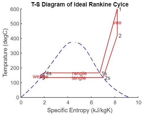
figure(1) % T-S
hold on
plot([S1 S2], [T1 T2], 'r', 'linewidth', 1)
text(S1,T1,' 1')
text(S2,T2,' 2')
plot([S2 S2g], [T2 T2s], 'r', 'linewidth', 1)
text(S2g,T2s,' 2s')
plot([S2g S3], [T2s T3], 'r', 'linewidth', 1)
text(S3,T3,' 3')
plot([S3 S4], [T3 T4], 'r', 'linewidth', 1)
text(S4,T4,' 4')
plot([S4 S1f], [T4 T1s], 'r', 'linewidth', 1)
text(S1f,T1s,' 4s')
plot([S1f S1g], [T1s T1s], 'r', 'linewidth', 1)
text(S1g,T1s,' 1s')
plot([S1g S1], [T1s T1], 'r', 'linewidth', 1)
plot(S_L, temp, 'b', 'linestyle','--','linewidth', 1)
plot(S_V, temp, 'b', 'linestyle','--','linewidth', 1)
%marking direction
text(S1,(T1+T2)/2,'vee','HorizontalAlignment','center','color','r')
text((S2g+S2f)/2,T3,'langle','color','r')
text(S3,(T3+T4)/2,'wedge','HorizontalAlignment','center','color','r')
text((S1f+S1g)/2,T1s,'rangle','color','r')
title('T-S Diagram of Ideal Rankine Cylce')
ylabel('Temprature (degC)')
xlabel('Specific Entropy (kJ/kgK)')
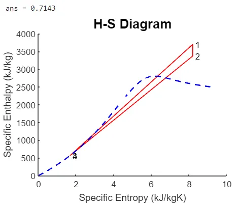
figure(2) % H-S
5/7
hold on
plot([S1 S2], [H1 H2], 'r', 'linewidth', 1);
text(S1,H1,' 1')
plot([S2 S3], [H2 H3], 'r', 'linewidth', 1);
text(S2,H2,' 2')
plot([S3 S4], [H3 H4], 'r', 'linewidth', 1);
text(S3,H3,' 3')
plot([S4 S1], [H4 H1], 'r', 'linewidth', 1);
text(S4,H4,' 4')
plot(S_L, H_L, 'b','linestyle','--', 'linewidth', 1.5)
plot(S_V, H_V, 'b','linestyle','--', 'linewidth', 1.5)
title('H-S Diagram', 'FontSize', 15)
ylabel('Specific Enthalpy (kJ/kg)')
xlabel('Specific Entropy (kJ/kgK)')
OUTPUT:
Enter the Pressure at the Turbine Inlet (in bar):
7
Enter the Temperature at the Turbine inlet (in Degree celsius):
600
Enter the Pressure at the Condenser (in bar):
3
SCREENCHOTS:
CODE EXPLANATION:
1.OPEN THE MATLAB ONLINE COMPILER AND TYPE CLEAR ALL , CLOSE ALL , CLC.
2.DOWNLOAD THE XSTEAM DATA AND IMPORT IT IN MATLAB.
3.THEN ENTER THE CODE FOR THE RANKINE CYCLE.
4.RUN THE CODE FOR THE OUTPUT.
5.PLOT THE T-S AND H-S IN THE MATLAB.
CONCLUSION:
THUS THE RANKINE CYCLE HAS BEEN SIMUATED USING MATLAB.