Project 2 - Rankine cycle Simulator
ANSWER:
Rankine Cycle:- The Rankine cycle is an idealized thermodynamic cycle describing the process by which certain heat engines, such as steam turbines or reciprocating steam engines, allow mechanical work to be extracted from a fluid as it moves between a heat source and heat sink.
Heat energy is supplied to the system via a boiler where the working fluid (typically water) is converted to a high pressure gaseous state (steam) in order to turn a turbine. After passing over the turbine the fluid is allowed to condense back into a liquid state as waste heat energy is rejected before being returned to boiler, completing the cycle. Friction losses throughout the system are often neglected for the purpose of simplifying calculations as such losses are usually much less significant than thermodynamic losses, especially in larger systems.
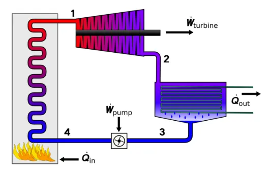
Layout of the Rankine cycle
- Turbine
- Condenser
- Pump
- Boiler
Processes and Working :
There are four processes in the rankine cycle (order maybe varied ) :
- Process 1-2 : Isentropic Expansion in the turbine .
- Process 2-3 : Constant pressure Heat rejection in condenser
- Process 3-4 : Isentropic compression in the pump
- Process 4-1 : Constant pressure heat addition in the boiler
Working of the rankine cycle simulator:
- In process 1-2 , The dry saturated vapour expands through a turbine, generating power. This decreases the temperature and pressure of the vapour, and some condensation may occur.
- Process 2-3 , The vapor-liquid mixture leaving the turbine (2) is condensed at low pressure, usually in a surface condenser using cooling water. In well designed and maintained condensers, the pressure of the vapor is well below atmospheric pressure, approaching the saturation pressure of the operating fluid at the cooling water temperature.
- Process 3-4 , The pressure of the condensate is raised in the feed pump. Because of the low specific volume of liquids, the pump work is relatively small and often neglected in thermodynamic calculations.
- Process 4-1 , High pressure liquid enters the boiler from the feed pump (4) and is heated to the saturation temperature (on the saturation curve). Further addition of energy causes evaporation of the liquid until it is fully converted to saturated steam (1) or superheated (1).
Formulae:-
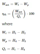
- Workdone & Efficiency
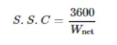
- Specific Stem Consuption
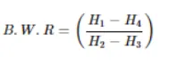
- Back Work Ratio
MATLAB CODE:
clearvars
close all
clc

%Process Information
fprintf('Rankine Cycle Simulator \n')
fprintf('process 1-2 : Isentropic Expansion \n')
fprintf('process 2-3 : Isobaric Heat Rejection \n')
fprintf('process 3-4 : Isentropic compression \n')
fprintf('process 4-1 : Isobaric heat addition process \n')

%Initial Inputs
P1 = input('Enter the inlet pressure of Turbine: ')
P2 = input('Enter the outlet pressure from Turbine: ')
T1 = input('Enter the steam inlet Temperature: ')

%State point 1
H1 = XSteam('h_pt',P1,T1); %Enthalpy
S1 = XSteam('s_pt',P1,T1); %Entropy
Hf1 = XSteam('hL_p',P1); %Enthalpy of saturated liquid
Hg1 = XSteam('hV_p',P1); %Enthalpy of saturated vapour
Ts1 = XSteam('Tsat_P',P1); %Saturation Temp
Sf1 = XSteam('sL_p',P1); %Entropy of saturated liquid
Sg1 = XSteam('sV_p',P1); %Entropy of saturated vapour

%State point 2
S2 = S1;
Sf2 = XSteam('sL_p',P2);
Sg2 = XSteam('sV_p',P2);
Hf2 = XSteam('hL_p',P2);
Hg2 = XSteam('hV_p',P2);
x = (S2-Sf2)/(Sg2-Sf2); %Dryness Fraction
H2 =Hf2+x*(Hg2-Hf2);
T2 = XSteam('T_ph',P2,H2);
Ts2= XSteam('Tsat_p',P2);

%State Point 3
H3 = Hf2;
S3 = Sf2;
T3 = T2;
P3 = P2;

%State point 4
P4 = P1;
S4 = S3;
H4 = XSteam('h_ps',P4,S4);
T4 = XSteam('T_Ps',P4,S4);

t = linspace(0,374,500);

%Plot T-S Diagram
figure(1)
hold on

for i = 1:length(t)
plot(XSteam('sL_T',t(i)),t(i),'.','color','b')
plot(XSteam('sV_T',t(i)),t(i),'.','color','b')
end

%Plot Cycle,
plot([S1,S2],[T1 T2],'linewidth',2,'color','r')
if x>1
T3 =Ts2;
plot([S2 Sg2 S3 S4],[T2,Ts2 T3 T4],'linewidth',2,'color','r')
T2 = Ts2;
else
plot([S2 S3 S4],[T2 T3 T4],'linewidth',2,'color','r');
end

l = linspace(T1,T2,1000)

for i=1:length(l)
plot(XSteam('s_pT',P1,l(i)),l(i),'.','color','r')
end
plot([Sf1 Sg1],[Ts1 Ts1],'linewidth',2,'color','r')
xlabel('Entropy[KJ/Kg-K]')
ylabel('Temprature[K]')
title('T-S Diagram')

%Plot H-S Diagram
figure(2)
hold on

%Plot Saturation Curve
for i=1:length(t)
plot(XSteam('sL_T',t(i)),XSteam('hL_T',t(i)),'.','color','b')
plot(XSteam('sV_T',t(i)),XSteam('hV_T',t(i)),'.','color','b')
end

%Plot Cycle
plot([S1 S2 S3 S4 S1],[H1 H2 H3 H4 H1],'linewidth',2,'color','r')
xlabel('Entropy[KJ/Kg-K]')
ylabel('Enthalpy[KJ/Kg]')
title('H-S Diagram')

%calcualtion

%Turbine Work
wt = H1-H2

%Pump Work
wp = H4-H3;

%Heat Addistion
Qin = H1-H4;

%Heat Rejection
Qout = H2-H3;

%Net Work
Wnet=wt-wp;

%Efficiency
Ntherm = (Wnet/Qin)*100

%Specific stem consumption
SSC = 3600/Wnet;

%Back power Ratio
BWR= wp/wt;

%Print Result
fprintf('\n\nResults\n')
fprintf('At State Point 1:\n')
fprintf('P1 is : %.2f bar\n',P1)
fprintf('T1 is : %.2f Deg Celcius\n',T1)
fprintf('H1 is : %.2f KJ/Kg\n',H1)
fprintf('S1 is : %.2f KJ/Kg-K\n',S1)

fprintf('\nAt State Point 2:\n')
fprintf('P2 is : %.2f bar\n',P2)
fprintf('T2 is : %.2f Deg Celcius\n',T2)
fprintf('H2 is : %.2f KJ/Kg\n',H2)
fprintf('S2 is : %.2f KJ/Kg-K\n',S2)

fprintf('\nAt State Point 3:\n')
fprintf('P3 is : %.2f bar\n',P3)
fprintf('T3 is : %.2f Deg Celcius\n',T3)
fprintf('H3 is : %.2f KJ/Kg\n',H3)
fprintf('S3 is : %.2f KJ/Kg-K\n',S3)

fprintf('\nAt State Point 4:\n')
fprintf('P4 is : %.2f bar\n',P4)
fprintf('T4 is : %.2f Deg Celcius\n',T4)
fprintf('H4 is : %.2f KJ/Kg\n',H4)
fprintf('S4 is : %.2f KJ/Kg-K\n',S4)

fprintf('\nWt is : %.2f KJ/Kg\n',wt)
fprintf('Wp is : %.2f KJ/Kg\n',wp)
fprintf('Wnet is : %.2f KJ/Kg\n', Wnet)
fprintf('Thermal Efficiency is : %.2f percent\n',Ntherm)
fprintf('S.S.C. is : %.2f Kg/KWh\n',SSC)
fprintf('Back Work Ratio is : %.3f \n',BWR)
Explaination:
- Clearvars, close all, clc, use to clear any previosly defined values.
- FIrst step is bring the given inputs to the program, for that the 'input()' command use. The user inputs includes tempareture and pressure entry to the turbine and pressue after existing to the turbine.
- Using the given inputs all four stages points are calculated.
- (H-Enthalpy, S-Entropy, T-Temperature, P-Pressure, x-Dryness factor, )
- After calculating all parameters, now calculate the Pumpwork, Turbine Work, Net work output, Back Ratio, Thermal Efficiency.
- Now to display all inputs 'fprintf()' command use.
- Next is to plot the grapt, H-S & T-S, First step to calculate the saturation curve for loop use.
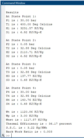
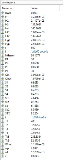
OUTPUT:
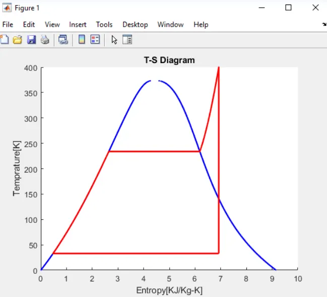
T-S PLOT:
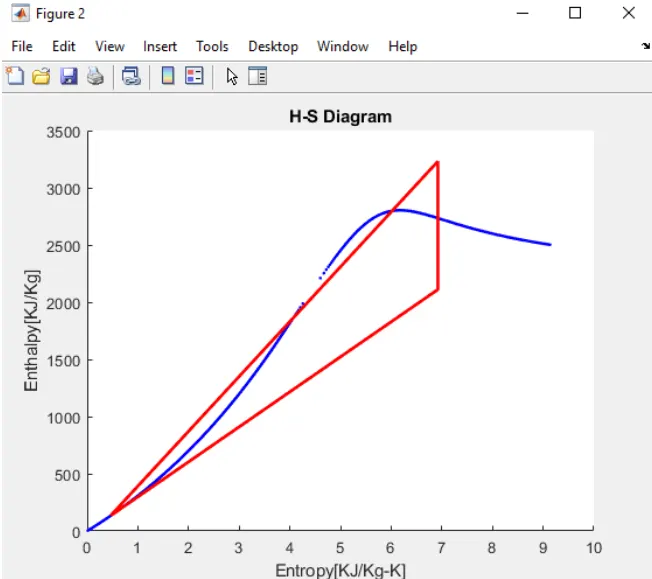
H-S PLOT:
CONCLUSION :
Based on inputs, we have calculated the state points of the Rankine Cycle using MATLAB. These plots are then matched up with the corresponding T-S and H-S plots for the given set of inputs. Also, its final result is shown in the command window.