Project 2 - EDA on Vehicle Insurance Customer Data
import pandas as pd
import numpy as np
import matplotlib.pyplot as plt
In [2]:
df1 = pd.read_csv("customer_details.csv")
df2 = pd.read_csv("customer_policy_details.csv")
In [3]:
col1=["Id","Gender","Age","Driving licence Active","regin code","Previously Insured","Vehical Age","Vehical Damage"]
df1.columns = col1
df1.head()
Out[3]:
| Id | Gender | Age | Driving licence Active | regin code | Previously Insured | Vehical Age | Vehical Damage | |
|---|---|---|---|---|---|---|---|---|
| 0 | 1.0 | Male | 44.0 | 1.0 | 28.0 | 0.0 | > 2 Years | Yes |
| 1 | 2.0 | Male | 76.0 | 1.0 | 3.0 | 0.0 | 1-2 Year | No |
| 2 | 3.0 | Male | 47.0 | 1.0 | 28.0 | 0.0 | > 2 Years | Yes |
| 3 | 4.0 | Male | 21.0 | 1.0 | 11.0 | 1.0 | < 1 Year | No |
| 4 | 5.0 | Female | 29.0 | 1.0 | 41.0 | 1.0 | < 1 Year | No |
In [4]:
col2 = ["Id","Anaual Salary","Sale channel code","Vintage","Response"]
df2.columns=col2
df2.head()
Out[4]:
| Id | Anaual Salary | Sale channel code | Vintage | Response | |
|---|---|---|---|---|---|
| 0 | 1.0 | 40454.0 | 26.0 | 217.0 | 1.0 |
| 1 | 2.0 | 33536.0 | 26.0 | 183.0 | 0.0 |
| 2 | 3.0 | 38294.0 | 26.0 | 27.0 | 1.0 |
| 3 | 4.0 | 28619.0 | 152.0 | 203.0 | 0.0 |
| 4 | 5.0 | 27496.0 | 152.0 | 39.0 | 0.0 |
In [5]:
df1_n = df1.isnull()
for i in df1_n.columns.values.tolist():
print(i)
print(df1_n[i].value_counts())
print("")
Id
False    380723
True        386
Name: Id, dtype: int64

Gender
False    380741
True        368
Name: Gender, dtype: int64

Age
False    380741
True        368
Name: Age, dtype: int64

Driving licence Active
False    380716
True        393
Name: Driving licence Active, dtype: int64

regin code
False    380717
True        392
Name: regin code, dtype: int64

Previously Insured
False    380728
True        381
Name: Previously Insured, dtype: int64

Vehical Age
False    380728
True        381
Name: Vehical Age, dtype: int64

Vehical Damage
False    380702
True        407
Name: Vehical Damage, dtype: int64
In [6]:
df2_n = df2.isnull()
for i in df2_n.columns.values.tolist():
print(i)
print(df2_n[i].value_counts())
print("")
Id
False    380722
True        387
Name: Id, dtype: int64

Anaual Salary
False    380763
True        346
Name: Anaual Salary, dtype: int64

Sale channel code
False    380709
True        400
Name: Sale channel code, dtype: int64

Vintage
False    380721
True        388
Name: Vintage, dtype: int64

Response
False    380748
True        361
Name: Response, dtype: int64
In [7]:
df1.dropna(subset=['Id'],axis = 0,inplace = True)
df1.reset_index(drop = True,inplace=True)
In [8]:
df2.dropna(subset=['Id'],axis = 0,inplace = True)
df2.reset_index(drop = True,inplace=True)
In [9]:
df1['Age'].fillna(df1['Age'].mean(),inplace=True)
In [10]:
df1['regin code'].fillna(df1['regin code'].mean(),inplace=True)
df1.head()
Out[10]:
| Id | Gender | Age | Driving licence Active | regin code | Previously Insured | Vehical Age | Vehical Damage | |
|---|---|---|---|---|---|---|---|---|
| 0 | 1.0 | Male | 44.0 | 1.0 | 28.0 | 0.0 | > 2 Years | Yes |
| 1 | 2.0 | Male | 76.0 | 1.0 | 3.0 | 0.0 | 1-2 Year | No |
| 2 | 3.0 | Male | 47.0 | 1.0 | 28.0 | 0.0 | > 2 Years | Yes |
| 3 | 4.0 | Male | 21.0 | 1.0 | 11.0 | 1.0 | < 1 Year | No |
| 4 | 5.0 | Female | 29.0 | 1.0 | 41.0 | 1.0 | < 1 Year | No |
In [11]:
df2['Anaual Salary'].fillna(df2['Anaual Salary'].mean(),inplace=True)
In [12]:
df2['Sale channel code'].fillna(df2['Sale channel code'].mean(),inplace=True)
In [13]:
df2['Vintage'].fillna(df2['Vintage'].mean(),inplace=True)
df2.head()
Out[13]:
| Id | Anaual Salary | Sale channel code | Vintage | Response | |
|---|---|---|---|---|---|
| 0 | 1.0 | 40454.0 | 26.0 | 217.0 | 1.0 |
| 1 | 2.0 | 33536.0 | 26.0 | 183.0 | 0.0 |
| 2 | 3.0 | 38294.0 | 26.0 | 27.0 | 1.0 |
| 3 | 4.0 | 28619.0 | 152.0 | 203.0 | 0.0 |
| 4 | 5.0 | 27496.0 | 152.0 | 39.0 | 0.0 |
In [14]:
df1['Driving licence Active'].fillna(df1['Driving licence Active'].mode()[0],inplace=True)
In [15]:
df1['Previously Insured'].fillna(df1['Previously Insured'].mode()[0],inplace=True)
df1.head()
Out[15]:
| Id | Gender | Age | Driving licence Active | regin code | Previously Insured | Vehical Age | Vehical Damage | |
|---|---|---|---|---|---|---|---|---|
| 0 | 1.0 | Male | 44.0 | 1.0 | 28.0 | 0.0 | > 2 Years | Yes |
| 1 | 2.0 | Male | 76.0 | 1.0 | 3.0 | 0.0 | 1-2 Year | No |
| 2 | 3.0 | Male | 47.0 | 1.0 | 28.0 | 0.0 | > 2 Years | Yes |
| 3 | 4.0 | Male | 21.0 | 1.0 | 11.0 | 1.0 | < 1 Year | No |
| 4 | 5.0 | Female | 29.0 | 1.0 | 41.0 | 1.0 | < 1 Year | No |
In [16]:
df2['Response'].fillna(df2['Response'].mode()[0],inplace=True)
df2.head()
Out[16]:
| Id | Anaual Salary | Sale channel code | Vintage | Response | |
|---|---|---|---|---|---|
| 0 | 1.0 | 40454.0 | 26.0 | 217.0 | 1.0 |
| 1 | 2.0 | 33536.0 | 26.0 | 183.0 | 0.0 |
| 2 | 3.0 | 38294.0 | 26.0 | 27.0 | 1.0 |
| 3 | 4.0 | 28619.0 | 152.0 | 203.0 | 0.0 |
| 4 | 5.0 | 27496.0 | 152.0 | 39.0 | 0.0 |
In [17]:
def plot_boxplot(df,ft):
df.boxplot(column=[ft])
plt.grid(False)
plt.show
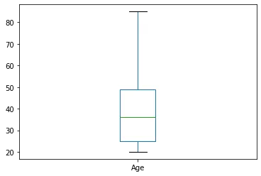
plot_boxplot(df1,'Age')
In [18]:
plot_boxplot(df1,'regin code')

In [19]:
def finding_out(df):
q1 = df.quantile(0.25)
q3=df.quantile(0.75)
iqr=q3-q1
outlier = df[((df<(q1-1.5*iqr)))|(df>(q3+1.5*iqr))]
return outlier
outliers = finding_out(df1['regin code'])
print("Number of outliers:",len(outliers))
print("Max Number of outliers:",outliers.max())
print("Minimum outlier value:",outliers.min())
Number of outliers: 0
Max Number of outliers: nan
Minimum outlier value: nan
In [20]:
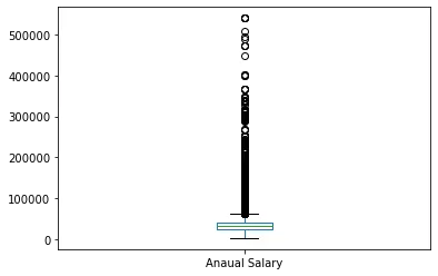
plot_boxplot(df2,'Anaual Salary')
In [21]:
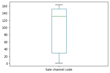
plot_boxplot(df2,'Sale channel code')
In [22]:
plot_boxplot(df2,'Vintage')

In [23]:
print("For Annual Salary")
outliers = finding_out(df2['Anaual Salary'])
print("Number of outliers:",len(outliers))
print("Max Number of outliers:",outliers.max())
print("Minimum outlier value:",outliers.min())
print('-**-'*16)
print("For sales channel code")
outliers = finding_out(df2['Sale channel code'])
print("Number of outliers:",len(outliers))
print("Max Number of outliers:",outliers.max())
print("Minimum outlier value:",outliers.min())
print('-**-'*16)
print("For Vintage")
outliers = finding_out(df2['Vintage'])
print("Number of outliers:",len(outliers))
print("Max Number of outliers:",outliers.max())
print("Minimum outlier value:",outliers.min())
print('-**-'*16)
For Annual Salary
Number of outliers: 10332
Max Number of outliers: 540165.0
Minimum outlier value: 61858.0
-**--**--**--**--**--**--**--**--**--**--**--**--**--**--**--**-
For sales channel code
Number of outliers: 0
Max Number of outliers: nan
Minimum outlier value: nan
-**--**--**--**--**--**--**--**--**--**--**--**--**--**--**--**-
For Vintage
Number of outliers: 0
Max Number of outliers: nan
Minimum outlier value: nan
-**--**--**--**--**--**--**--**--**--**--**--**--**--**--**--**-
In [24]:
def replace(df):
q1 = df.quantile(0.25)
q3=df.quantile(0.75)
iqr=q3-q1
upper = df[~(df>(q3+1.5*iqr))].max()
lower = df[~(df>(q3+1.5*iqr))].min()
return df
replace(df2['Anaual Salary'])
Out[24]:
0         40454.0
1         33536.0
2         38294.0
3         28619.0
4         27496.0
           ...
380717    30170.0
380718    40016.0
380719    35118.0
380720    44617.0
380721    41777.0
Name: Anaual Salary, Length: 380722, dtype: float64
In [25]:
df1.apply(lambda x:x.str.strip() if x.dtype == 'object'else x)
Out[25]:
| Id | Gender | Age | Driving licence Active | regin code | Previously Insured | Vehical Age | Vehical Damage | |
|---|---|---|---|---|---|---|---|---|
| 0 | 1.0 | Male | 44.0 | 1.0 | 28.0 | 0.0 | > 2 Years | Yes |
| 1 | 2.0 | Male | 76.0 | 1.0 | 3.0 | 0.0 | 1-2 Year | No |
| 2 | 3.0 | Male | 47.0 | 1.0 | 28.0 | 0.0 | > 2 Years | Yes |
| 3 | 4.0 | Male | 21.0 | 1.0 | 11.0 | 1.0 | < 1 Year | No |
| 4 | 5.0 | Female | 29.0 | 1.0 | 41.0 | 1.0 | < 1 Year | No |
| ... | ... | ... | ... | ... | ... | ... | ... | ... |
| 380718 | 381105.0 | Male | 74.0 | 1.0 | 26.0 | 1.0 | 1-2 Year | No |
| 380719 | 381106.0 | Male | 30.0 | 1.0 | 37.0 | 1.0 | < 1 Year | No |
| 380720 | 381107.0 | Male | 21.0 | 1.0 | 30.0 | 1.0 | < 1 Year | No |
| 380721 | 381108.0 | Female | 68.0 | 1.0 | 14.0 | 0.0 | > 2 Years | Yes |
| 380722 | 381109.0 | Male | 46.0 | 1.0 | 29.0 | 0.0 | 1-2 Year | No |
380723 rows × 8 columns
In [26]:
df1.apply(lambda x:x.str.upper() if x.dtype == 'object'else x)
Out[26]:
| Id | Gender | Age | Driving licence Active | regin code | Previously Insured | Vehical Age | Vehical Damage | |
|---|---|---|---|---|---|---|---|---|
| 0 | 1.0 | MALE | 44.0 | 1.0 | 28.0 | 0.0 | > 2 YEARS | YES |
| 1 | 2.0 | MALE | 76.0 | 1.0 | 3.0 | 0.0 | 1-2 YEAR | NO |
| 2 | 3.0 | MALE | 47.0 | 1.0 | 28.0 | 0.0 | > 2 YEARS | YES |
| 3 | 4.0 | MALE | 21.0 | 1.0 | 11.0 | 1.0 | < 1 YEAR | NO |
| 4 | 5.0 | FEMALE | 29.0 | 1.0 | 41.0 | 1.0 | < 1 YEAR | NO |
| ... | ... | ... | ... | ... | ... | ... | ... | ... |
| 380718 | 381105.0 | MALE | 74.0 | 1.0 | 26.0 | 1.0 | 1-2 YEAR | NO |
| 380719 | 381106.0 | MALE | 30.0 | 1.0 | 37.0 | 1.0 | < 1 YEAR | NO |
| 380720 | 381107.0 | MALE | 21.0 | 1.0 | 30.0 | 1.0 | < 1 YEAR | NO |
| 380721 | 381108.0 | FEMALE | 68.0 | 1.0 | 14.0 | 0.0 | > 2 YEARS | YES |
| 380722 | 381109.0 | MALE | 46.0 | 1.0 | 29.0 | 0.0 | 1-2 YEAR | NO |
380723 rows × 8 columns
In [27]:
dummy_variable_1 = pd.get_dummies(df1['Vehical Damage'])
dummy_variable_1.rename(columns={'No':'vehicale-damage-No','Yes':'vehicle-damage-Yes'},inplace = True)
dummy_variable_1.head()
Out[27]:
| vehicale-damage-No | vehicle-damage-Yes | |
|---|---|---|
| 0 | 0 | 1 |
| 1 | 1 | 0 |
| 2 | 0 | 1 |
| 3 | 1 | 0 |
| 4 | 1 | 0 |
In [33]:
master_data = pd.merge(df1,df2,on='Id')
master_data
Out[33]:
| Id | Gender | Age | Driving licence Active | regin code | Previously Insured | Vehical Age | Vehical Damage | Anaual Salary | Sale channel code | Vintage | Response | |
|---|---|---|---|---|---|---|---|---|---|---|---|---|
| 0 | 1.0 | Male | 44.0 | 1.0 | 28.0 | 0.0 | > 2 Years | Yes | 40454.0 | 26.0 | 217.0 | 1.0 |
| 1 | 2.0 | Male | 76.0 | 1.0 | 3.0 | 0.0 | 1-2 Year | No | 33536.0 | 26.0 | 183.0 | 0.0 |
| 2 | 3.0 | Male | 47.0 | 1.0 | 28.0 | 0.0 | > 2 Years | Yes | 38294.0 | 26.0 | 27.0 | 1.0 |
| 3 | 4.0 | Male | 21.0 | 1.0 | 11.0 | 1.0 | < 1 Year | No | 28619.0 | 152.0 | 203.0 | 0.0 |
| 4 | 5.0 | Female | 29.0 | 1.0 | 41.0 | 1.0 | < 1 Year | No | 27496.0 | 152.0 | 39.0 | 0.0 |
| ... | ... | ... | ... | ... | ... | ... | ... | ... | ... | ... | ... | ... |
| 380331 | 381105.0 | Male | 74.0 | 1.0 | 26.0 | 1.0 | 1-2 Year | No | 30170.0 | 26.0 | 88.0 | 0.0 |
| 380332 | 381106.0 | Male | 30.0 | 1.0 | 37.0 | 1.0 | < 1 Year | No | 40016.0 | 152.0 | 131.0 | 0.0 |
| 380333 | 381107.0 | Male | 21.0 | 1.0 | 30.0 | 1.0 | < 1 Year | No | 35118.0 | 160.0 | 161.0 | 0.0 |
| 380334 | 381108.0 | Female | 68.0 | 1.0 | 14.0 | 0.0 | > 2 Years | Yes | 44617.0 | 124.0 | 74.0 | 0.0 |
| 380335 | 381109.0 | Male | 46.0 | 1.0 | 29.0 | 0.0 | 1-2 Year | No | 41777.0 | 26.0 | 237.0 | 0.0 |
380336 rows × 12 columns
In [34]:
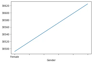
all_data = master_data.groupby('Gender')['Anaual Salary'].mean()
all_data
Out[34]:
Gender
Female    30492.028478
Male      30624.622150
Name: Anaual Salary, dtype: float64
In [35]:
all_data.plot()
Out[35]:
<AxesSubplot:xlabel='Gender'>
In [36]:
all_data.plot.bar(title='Gender vs Annual Salary')
Out[36]:
<AxesSubplot:title={'center':'Gender vs Annual Salary'}, xlabel='Gender'>

In [37]:
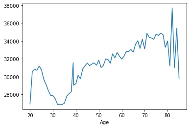
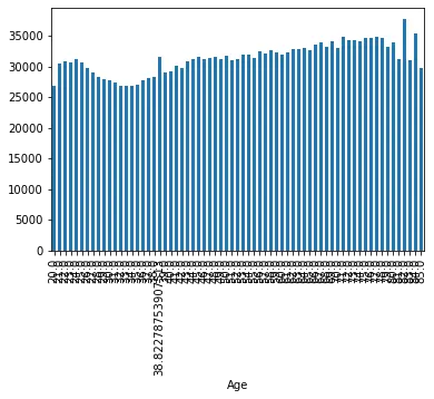
age_data =master_data.groupby('Age')['Anaual Salary'].mean()
age_data
Out[37]:
Age
20.0    26924.620173
21.0    30564.475810
22.0    30823.778102
23.0    30688.606298
24.0    31183.802890
            ...
81.0    31201.571429
82.0    37705.379310
83.0    31012.727273
84.0    35440.818182
85.0    29792.363636
Name: Anaual Salary, Length: 67, dtype: float64
In [38]:
age_data.plot()
Out[38]:
<AxesSubplot:xlabel='Age'>
In [39]:
age_data.plot.bar()
Out[39]:
<AxesSubplot:xlabel='Age'>
In [40]:
master_data.groupby('Gender').count()
Out[40]:
| Id | Age | Driving licence Active | regin code | Previously Insured | Vehical Age | Vehical Damage | Anaual Salary | Sale channel code | Vintage | Response | |
|---|---|---|---|---|---|---|---|---|---|---|---|
| Gender | |||||||||||
| Female | 174485 | 174485 | 174485 | 174485 | 174485 | 174309 | 174300 | 174485 | 174485 | 174485 | 174485 |
| Male | 205484 | 205484 | 205484 | 205484 | 205484 | 205279 | 205266 | 205484 | 205484 | 205484 | 205484 |
In [41]:
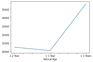
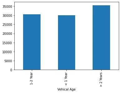
vehical_age =master_data.groupby('Vehical Age')['Anaual Salary'].mean()
vehical_age
Out[41]:
Vehical Age
1-2 Year     30522.464972
< 1 Year     30115.716367
> 2 Years    35657.520845
Name: Anaual Salary, dtype: float64
In [42]:
vehical_age.plot()
Out[42]:
<AxesSubplot:xlabel='Vehical Age'>
In [43]:
vehical_age.plot.bar()
Out[43]:
<AxesSubplot:xlabel='Vehical Age'>
In [44]:
master_data['Age'].corr(master_data['Anaual Salary'])
Out[44]:
0.0677151598661391
In [45]:
master_data[['Age','Anaual Salary']].corr()
Out[45]:
| Age | Anaual Salary | |
|---|---|---|
| Age | 1.000000 | 0.067715 |
| Anaual Salary | 0.067715 | 1.000000 |