Basics of ML & AL Week 2 Challenge

# Question 1

# Question 2

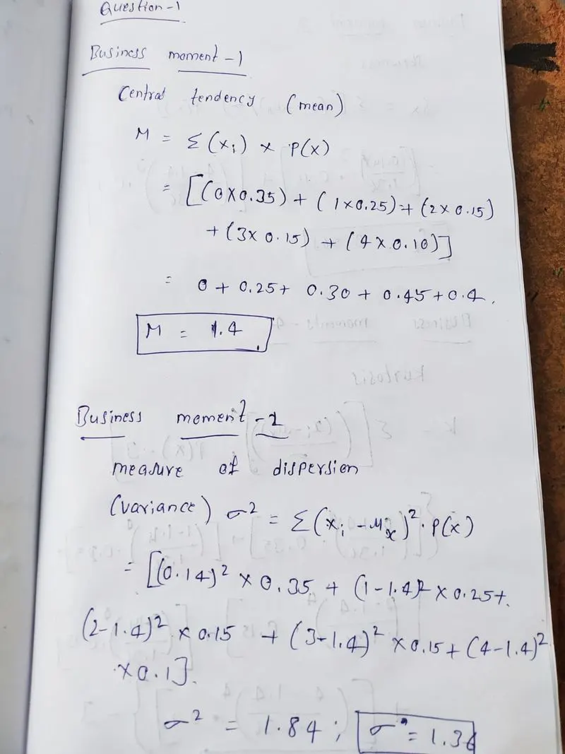
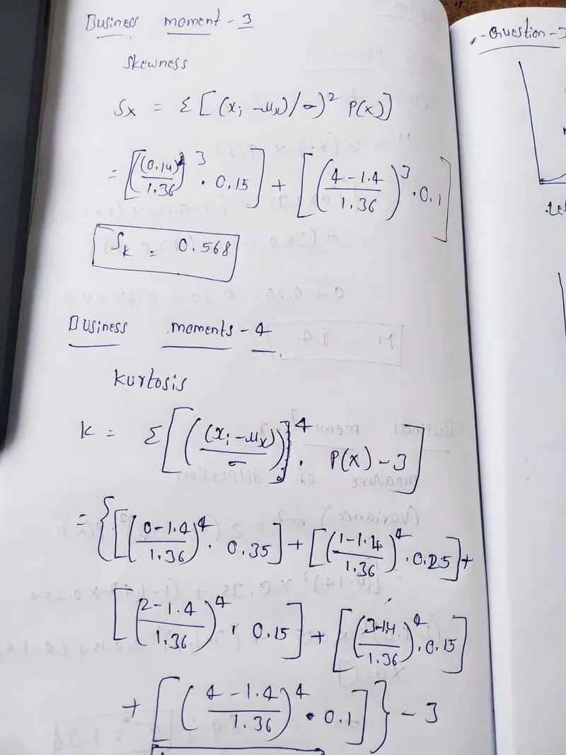
It is true that simple mean is sufficient enough for having an idea about the data by computing with its formula ( sum of all observations/number of observations). But, by foregoing this computation we assume that the possibility of each event happening is equal and hence we directly compute them by summing them and taking their average. But, What if the occurance of all the events arent given? Assume we have 4 events possibly to occur namely A B and C.

So we arent given with their number of occurance in definite numbers say, A happens for 4 times, B happens for 8 times and so on. For this scenario simple mean itself is enough. But, whatif instead of their number of occurance, their probability of B to occur is 0.31 and for C 0.21. This would get us to a point where we need to consider the weight of the event. This would get us to a point where we need to consider the weight of the event. As given in the example above, the probability of A is more than B and C. That means when we correlate this with its occurance, we can infer that the mean or the ideal possibility of the event to occur would be closest to that of A and father from C (Holding the least probability) imagine having more random variables and complex probability values. That is when the significance of expected mean value overcomes the simple mean value. As explained in the previous question, instead of summing the probability, we should consider the weight of each event before averaging them.

Note: The sum of the probabilities should always be 1.

# Question 3

One cannot determine whether having skewness is a good thing or not. Because different types of skewness depicts the data according to the domain of its application.

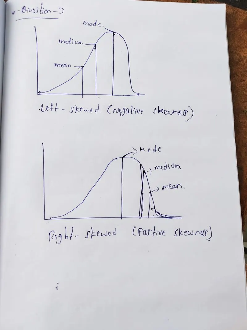
In the imagine given above two different types of skewness has been showed. In the left skewed graph, an example of this type of graph would time at which most of the school closes. Many schools close around 3pm - 5pm. So the median value would be close to the right side of the graph if we were to plot from 10am to 7pm in the x-axis.

Similarly, for the right skewed graph, an example would be that of a vehicle speed going on a road in the city traffic. Most people would drive with a speed of 30 - 40km/hr where the x-axis ranges from 0-100km/hr range.

so, according to the given data, the skewness makes sense for that particular data and not every graph could be symmetrical on both sides for a real time dataset.

# Question 4

To evaluate the probability value for continous normal distribution, we calculate the z-score with the given mean and standard variation for each of the data point given by the formula,

z-score = (x - mean) / standard deviation.

Then the z values are looked into the corresponding z-table to identify the probability less than or equal to that value.

For the given data points we have,

1.P(X<711)

The z-score of this would be = (711-680)/31 = 1.

Hence, it is one standard deviation away from the mean in the positive x axis.

In the z-table, the probability value for z= +1 is 0.8413 which is 84.13%.

2.P(X>740)

The z-score of this would be = (740-680)/31 = 1.93.

Hence, it us 1.9 times the standard deviation away from the mean mean in the positive x axis.

In thw z-table, the probability value for z = +1.93 which is 0.9732.

But it is asked for probability greater than 740. Hence, we get the value until 740 and subtract from 1.

so, the final probability value = 1 - 0.9732 = 0.0268 or 2.68%.

3.P(600

In this case, we need to find the value of probability at X < 720 and X<600 and subtract both values.

When X = 720, z = 1.29 and probability value is 0.9015

When X = 600, z = -2.58 and probability value is 0.00494

Final probability value = 0.9015 - 0.00494 = 0.89656 or 89.656%.

4.P(X=720)

P(z = 1.29) = P(Z<1.29) - P(Z < 1.29)

P(z = 1.29) = 0.9032 - 0.9032

P(Z = 1.29) = 0.

# Question 5

The graph given below shows the normal distribution of the data points by plotting the z - values with their corresponding probability values.

Here, the mean of this observation data is always 0 and the standard deviation is 1.

It gives us the percentage of data falling under every 1,2, and 3 standard deviation from the mean value.

In this figure, 68.2% of data falls from z values -1 to +1, 95.4% from -2 to +2 and 99.6% from -3 to +3.

An example application of this graph would be the results of IQ test of people living in a city.

It can be noted that not everyone would have gotten the highest IQ or the lowest. Most of the range would be around the mean value which is depicted by this graph. Another example would be marks obtained in a test. It can be observed that people who score centum and people who scored a zero would be very less. More students marks would be around the average class mark.