Project 2 - EDA on Vehicle Insurance Customer Data
EDA on Vehicle Insurance Customer Data
In [1]:
# Reading Data
import pandas as pd
DF1 = pd.read_csv("customer_details.csv")
DF2 = pd.read_csv("customer_policy_details.csv")
print(DF1.head())
print(DF2.head())
     0       1     2    3     4    5          6    7
0  1.0    Male  44.0  1.0  28.0  0.0  > 2 Years  Yes
1  2.0    Male  76.0  1.0   3.0  0.0   1-2 Year   No
2  3.0    Male  47.0  1.0  28.0  0.0  > 2 Years  Yes
3  4.0    Male  21.0  1.0  11.0  1.0   < 1 Year   No
4  5.0  Female  29.0  1.0  41.0  1.0   < 1 Year   No
     0        1      2      3    4
0  1.0  40454.0   26.0  217.0  1.0
1  2.0  33536.0   26.0  183.0  0.0
2  3.0  38294.0   26.0   27.0  1.0
3  4.0  28619.0  152.0  203.0  0.0
4  5.0  27496.0  152.0   39.0  0.0
In [2]:
# 1. Add the column names to both datasets:
# i. Column Name for customer details table:
#File1(customer_details)
DF1.columns=['customer_id','gender','age','driving_liscence_present','region_code','previously_insured','vehicle_age','vehicle_damage']
# ii. Column Name for customer_policy table:
#File2(customer_policy_details)
DF2.columns=['customer_id','annual_premium','sales_channel_code','vintage','response']
In [3]:
# 2. Checking and Cleaning Data Quality:
# 2.i(a)Generate a summary of count of all the null values column wise
# File1(customer_details)
print(DF1.isnull().sum())
print('*'*50)
#File2(customer_policy_details)
print(DF2.isnull().sum())
customer_id                 386
gender                      368
age                         368
driving_liscence_present    393
region_code                 392
previously_insured          381
vehicle_age                 381
vehicle_damage              407
dtype: int64
**************************************************
customer_id           387
annual_premium        346
sales_channel_code    400
vintage               388
response              361
dtype: int64
In [4]:
# 2.i(b)Drop Null values for customer_id because central tendencies for id’s is not feasible.
#File1(customer_details)
DF1.dropna(subset=['customer_id'],inplace=True)
print(DF1.isnull().sum())
print('*'*50)
#File2(customer_policy_details)
DF2.dropna(subset=['customer_id'],inplace=True)
print(DF2.isnull().sum())
customer_id                   0
gender                      368
age                         366
driving_liscence_present    392
region_code                 391
previously_insured          381
vehicle_age                 381
vehicle_damage              406
dtype: int64
**************************************************
customer_id             0
annual_premium        344
sales_channel_code    400
vintage               388
response              361
dtype: int64
In [5]:
# 2.i(c)Replace all null values for numeric columns by mean.
#File1(customer_details)
for column in DF1[['age', 'driving_liscence_present', 'region_code','previously_insured']]:
mean = DF1[column].mean()
DF1[column] = DF1[column].fillna(mean)
print('_'*100)
#File2(customer_policy_details)
for column in DF2[['annual_premium','sales_channel_code','vintage','response']]:
mean = DF2[column].mean()
DF2[column] = DF2[column].fillna(mean)
____________________________________________________________________________________________________
In [6]:
# 2.i(d)Replace all null values for Categorical value by mode.
#File1(customer_details)
for column in DF1[['gender', 'vehicle_age', 'vehicle_damage']]:
mode = DF1[column].mode()
DF1[column] = DF1[column].fillna(mode)
In [7]:
#2.ii Outliers
# 2.ii(a) Generate a summary of count of all the outliers column wise
#File1(customer_details)
DF1['age'].describe()
DF1['driving_liscence_present'].describe()
DF1['previously_insured'].describe()
DF1['region_code'].describe()
#File2(customer_policy_details)
DF2['annual_premium'].describe()
DF2['sales_channel_code'].describe()
DF2['vintage'].describe()
DF2['response'].describe()
Out[7]:
count    380722.000000
mean          0.122526
std           0.327737
min           0.000000
25%           0.000000
50%           0.000000
75%           0.000000
max           1.000000
Name: response, dtype: float64
In [8]:
# 2.ii (b) Replace all outlier values for numeric columns by mean.
In [9]:
# 2.iii. White spaces
# Remove white spaces
#File1(customer_details)
DF1.apply(lambda x: x.str.strip() if x.dtype=="object" else x)
print('*'*50)
#File2(customer_policy_details)
DF2.apply(lambda x: x.str.strip() if x.dtype=="object" else x)
**************************************************
Out[9]:
| customer_id | annual_premium | sales_channel_code | vintage | response | |
|---|---|---|---|---|---|
| 0 | 1.0 | 40454.0 | 26.0 | 217.0 | 1.0 |
| 1 | 2.0 | 33536.0 | 26.0 | 183.0 | 0.0 |
| 2 | 3.0 | 38294.0 | 26.0 | 27.0 | 1.0 |
| 3 | 4.0 | 28619.0 | 152.0 | 203.0 | 0.0 |
| 4 | 5.0 | 27496.0 | 152.0 | 39.0 | 0.0 |
| ... | ... | ... | ... | ... | ... |
| 381104 | 381105.0 | 30170.0 | 26.0 | 88.0 | 0.0 |
| 381105 | 381106.0 | 40016.0 | 152.0 | 131.0 | 0.0 |
| 381106 | 381107.0 | 35118.0 | 160.0 | 161.0 | 0.0 |
| 381107 | 381108.0 | 44617.0 | 124.0 | 74.0 | 0.0 |
| 381108 | 381109.0 | 41777.0 | 26.0 | 237.0 | 0.0 |
380722 rows × 5 columns
In [10]:
# 2.iv. case correction(lower or upper, any one)
#File1(customer_details)
DF1.apply(lambda x: x.str.lower() if x.dtype == "object" else x)
print('*'*100)
#File2(customer_policy_details)
DF2.apply(lambda x: x.str.lower() if x.dtype == "object" else x)
****************************************************************************************************
Out[10]:
| customer_id | annual_premium | sales_channel_code | vintage | response | |
|---|---|---|---|---|---|
| 0 | 1.0 | 40454.0 | 26.0 | 217.0 | 1.0 |
| 1 | 2.0 | 33536.0 | 26.0 | 183.0 | 0.0 |
| 2 | 3.0 | 38294.0 | 26.0 | 27.0 | 1.0 |
| 3 | 4.0 | 28619.0 | 152.0 | 203.0 | 0.0 |
| 4 | 5.0 | 27496.0 | 152.0 | 39.0 | 0.0 |
| ... | ... | ... | ... | ... | ... |
| 381104 | 381105.0 | 30170.0 | 26.0 | 88.0 | 0.0 |
| 381105 | 381106.0 | 40016.0 | 152.0 | 131.0 | 0.0 |
| 381106 | 381107.0 | 35118.0 | 160.0 | 161.0 | 0.0 |
| 381107 | 381108.0 | 44617.0 | 124.0 | 74.0 | 0.0 |
| 381108 | 381109.0 | 41777.0 | 26.0 | 237.0 | 0.0 |
380722 rows × 5 columns
In [11]:
# 2.v. Convert nominal data (categorical) into dummies
# for future modeling use if required
#File1(customer_details)
DF1_dummies = pd.get_dummies(DF1, columns=['gender'])
DF1_dummies.head()
#File2(customer_policy_details)
DF2_dummies = pd.get_dummies(DF2, columns=['response'])
DF2_dummies.head()
Out[11]:
| customer_id | annual_premium | sales_channel_code | vintage | response_0.0 | response_0.12252570584260741 | response_1.0 | |
|---|---|---|---|---|---|---|---|
| 0 | 1.0 | 40454.0 | 26.0 | 217.0 | 0 | 0 | 1 |
| 1 | 2.0 | 33536.0 | 26.0 | 183.0 | 1 | 0 | 0 |
| 2 | 3.0 | 38294.0 | 26.0 | 27.0 | 0 | 0 | 1 |
| 3 | 4.0 | 28619.0 | 152.0 | 203.0 | 1 | 0 | 0 |
| 4 | 5.0 | 27496.0 | 152.0 | 39.0 | 1 | 0 | 0 |
In [12]:
# 2.vi. Drop Duplicates (duplicated rows)
#File1(customer_details)
DF1.drop_duplicates(inplace=True)
#File2(customer_policy_details)
DF2.drop_duplicates(inplace=True)
In [13]:
# 3.Create a Master table for future use.
# Join the customer table and customer_policy table to get a master table using customer_id in both tables.
# (Hint: use pd.merge() function)
data=pd.merge(DF1,DF2,on='customer_id')
data
Out[13]:
| customer_id | gender | age | driving_liscence_present | region_code | previously_insured | vehicle_age | vehicle_damage | annual_premium | sales_channel_code | vintage | response | |
|---|---|---|---|---|---|---|---|---|---|---|---|---|
| 0 | 1.0 | Male | 44.0 | 1.0 | 28.0 | 0.0 | > 2 Years | Yes | 40454.0 | 26.0 | 217.0 | 1.0 |
| 1 | 2.0 | Male | 76.0 | 1.0 | 3.0 | 0.0 | 1-2 Year | No | 33536.0 | 26.0 | 183.0 | 0.0 |
| 2 | 3.0 | Male | 47.0 | 1.0 | 28.0 | 0.0 | > 2 Years | Yes | 38294.0 | 26.0 | 27.0 | 1.0 |
| 3 | 4.0 | Male | 21.0 | 1.0 | 11.0 | 1.0 | < 1 Year | No | 28619.0 | 152.0 | 203.0 | 0.0 |
| 4 | 5.0 | Female | 29.0 | 1.0 | 41.0 | 1.0 | < 1 Year | No | 27496.0 | 152.0 | 39.0 | 0.0 |
| ... | ... | ... | ... | ... | ... | ... | ... | ... | ... | ... | ... | ... |
| 380331 | 381105.0 | Male | 74.0 | 1.0 | 26.0 | 1.0 | 1-2 Year | No | 30170.0 | 26.0 | 88.0 | 0.0 |
| 380332 | 381106.0 | Male | 30.0 | 1.0 | 37.0 | 1.0 | < 1 Year | No | 40016.0 | 152.0 | 131.0 | 0.0 |
| 380333 | 381107.0 | Male | 21.0 | 1.0 | 30.0 | 1.0 | < 1 Year | No | 35118.0 | 160.0 | 161.0 | 0.0 |
| 380334 | 381108.0 | Female | 68.0 | 1.0 | 14.0 | 0.0 | > 2 Years | Yes | 44617.0 | 124.0 | 74.0 | 0.0 |
| 380335 | 381109.0 | Male | 46.0 | 1.0 | 29.0 | 0.0 | 1-2 Year | No | 41777.0 | 26.0 | 237.0 | 0.0 |
380336 rows × 12 columns
In [14]:
# 4. Company needs some important information from the master table to make decisions for future growth.
# They needs following information:
# 4.i Gender wise average annual premium
data.groupby('gender')['annual_premium'].mean()
# 4.ii. Age wise average annual premium
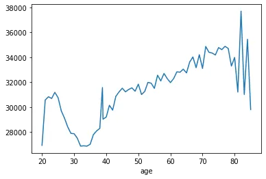
result = data.groupby('age')['annual_premium'].mean()
import matplotlib.pyplot as pyplot
result.plot()
pyplot.show()
# 4.iii. Is your data balanced between the genders?
# (Hint: Data is balanced if number of counts in each group is approximately same)
print(f"male to female ration is {round(data['gender'].value_counts()[0]/data['gender'].value_counts()[1],2)}")
print(f"generally, the standard is: \n balanced data ratio: {50/50}\n slightly balanced data ratio: {round(55/45,2)}-{60/40} \n imbalanced data ratio: {80/20}-{90/10}")
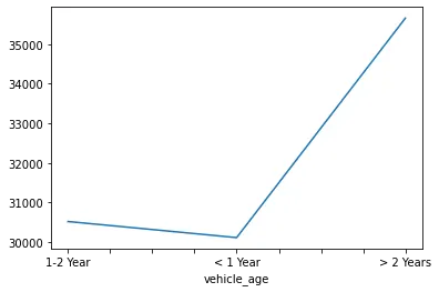
# 4.iv. Vehicle age wise average annual premium.
result1 = data.groupby('vehicle_age')['annual_premium'].mean()
import matplotlib.pyplot as pyplot
result1.plot()
pyplot.show()
male to female ration is 1.18
generally, the standard is:
 balanced data ratio: 1.0
 slightly balanced data ratio: 1.22-1.5
 imbalanced data ratio: 4.0-9.0
In [15]:
# 5.Is there any relation between Person Age and annual premium?
# Hint: use correlation function (Correlation describes the relationship between two variables).
# Correlation coefficient < -0.5 - Strong negative relationship
# Correlation coefficient > 0.5 - Strong positive relationship
# 0.5 < Correlation coefficient < 0.5 - There is no relationship.
n = data['age'].corr(data['annual_premium'])
if n<-0.5:
print("Strong negative relationship")
if n>0.5:
print("Strong positive relationship")
if n>-0.5 and n<0.5:
print("There is no relationship!")
There is no relationship!