Project 2
Aim:
Development of a forward energy-based fuel consumption model of a Hybrid vehicle.
Objective:
- Tabulate the fuel economy numbers (kmpl) for UDDS and HWFET cycle. This forms the baseline numbers for comparing with the conventional vehicle model.
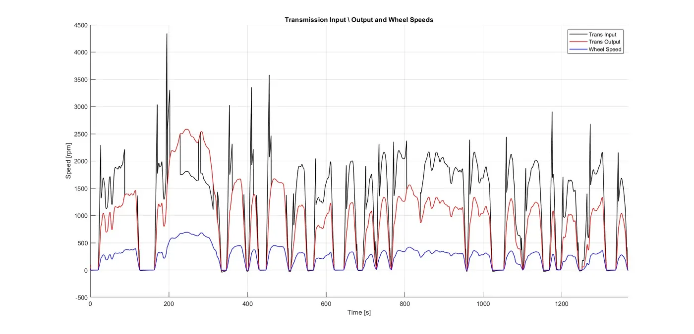
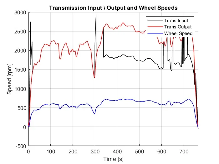
- Plot the time trace for engine, transmission input, transmission output and wheel speed on one plot.
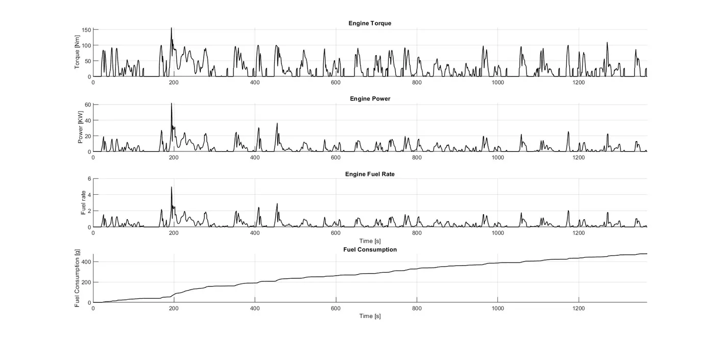
- Plot engine torque, engine power, fuel rate and fuel consumption using subplots.
- Plot accelerator and brake pedal, gear command, vehicle desired and actual speed, vehicle distance using subplots.
- Plot the engine operating points on the engine fuel map.
- Plot motor speed, torque, motor input power using subplots.
- Plot pack voltage, current and SoC using subplots.
- Plot the motor operating points on the motor input power map, with the motor max motoring and generating torque curves.
- Write down appropriate brief comments on each of these plots, describing the vehicle behavior throughout the drive cycle.
- Generate the plots for both drive cycles.
Introduction –
A hybrid vehicle is one that uses two or more distinct types of power, such as Gasoline or diesel and batteries. Like submarines that use diesel when surfaced and batteries when submerged. Hybrid powertrains are designed to switch from one power source to another to maximize both fuel efficiency and energy efficiency. In hybrid electric vehicles, for instance, the electric motor is more efficient at producing torque, or turning power, while the combustion engine is better for maintaining high speed. Improved efficiency, lower emissions, and reduced running costs relative to non-hybrid vehicles are three primary benefits of hybridization.
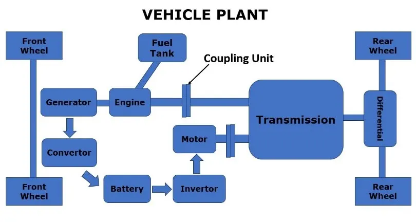
Forward model of Hybrid vehicle:
The forward modelling is also known as cause-effect, engine-to-wheel or rear-to-front method. The direction of calculation is the same as the direction of positive power flow which is from engine to wheels.
A forward-facing vehicle model features a driver model that provides torque demand in the form of a desired ICE torque and brake torque, to meet the speed trace from a drive cycle. A basic driver model typically uses one or more Proportional- Integral (PI) controllers to achieve the torque demand, with reference to the desired speed trace. The torque produced by the ICE propagates through the transmission and final drive ratios, before ending up as torque applied at the wheels. This is then exerted to the vehicle mass via force on the tyre contact patch. The vehicle speed that results from the applied force is propagated back through the drivetrain, and returns to the ICE as angular velocity at the crankshaft. Brake torque is applied directly at the wheels.
This
model can be used to compare the fuel efficiency of different vehicles, or to
identify opportunities for improving the fuel efficiency of a particular
vehicle. For example, if you are trying to improve the fuel efficiency of a
vehicle, you could modify its design or driving behavior to reduce its energy
consumption, and then use the forward energy-based fuel consumption model to
estimate the resulting improvement in fuel efficiency.
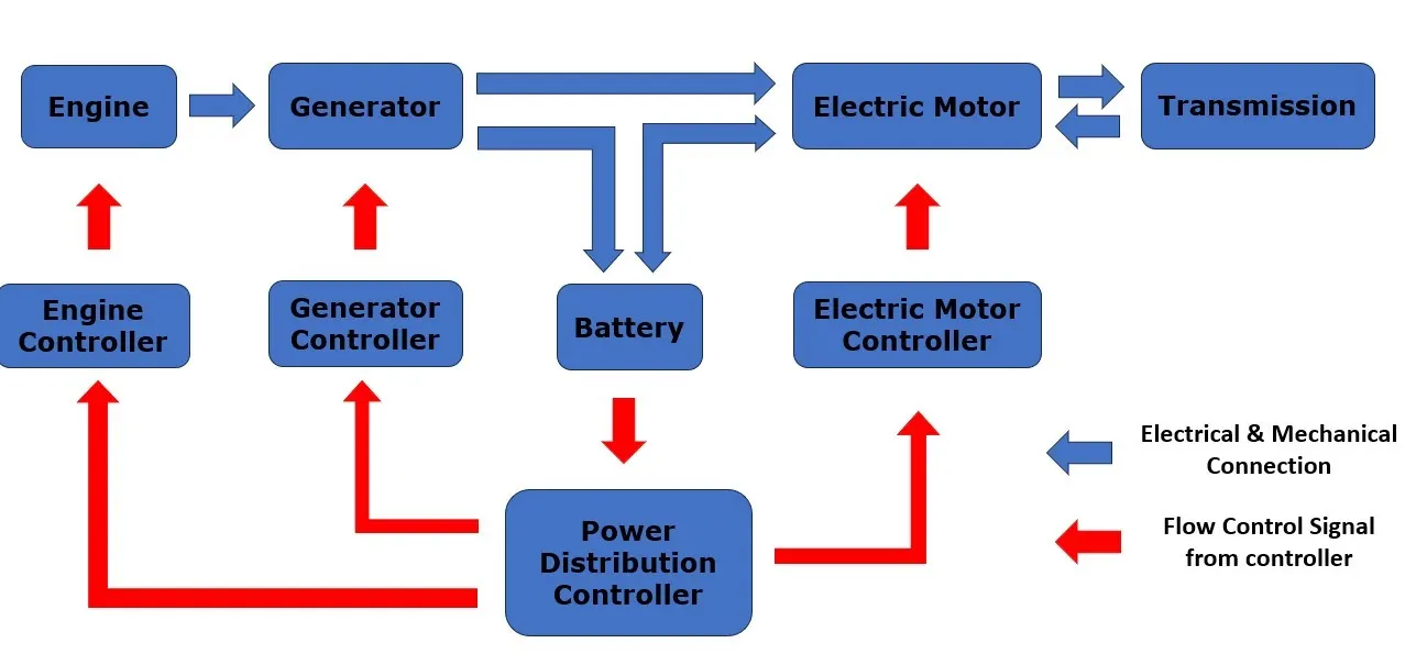
Hybrid
Powertrain Efficiency:
For normal steady state operating condition, hybridization gives an extra degree of freedom to allow the engine to operate at the peak efficiency point.
As transmissions give the degree of freedom to change the operating condition subject to same power input, hybridization gives extra degree of freedom to change the operating power if the engine keeping the same output power.
For Hybrid vehicle, the wheel power is supplied either by engine or motor through the transmission drivetrain,
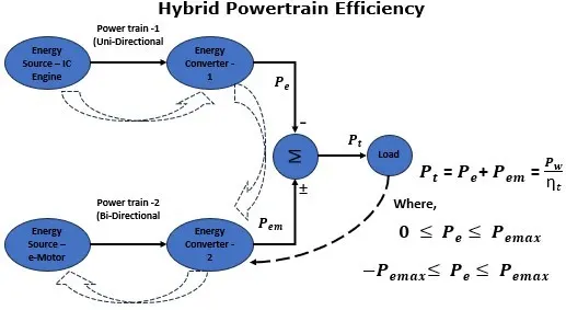
The power for electric motor comes from the electric energy stored in the battery. The direction of power flow depends on whether energy is being drawn from or supplied to the battery by the electric drive unit.
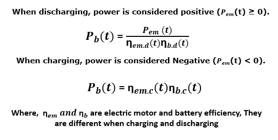
Now, for pure hybrid electric vehicle, the vehicle battery cannot be charged by an external energy source. This is known as charge-sustaining strategy, where charge in battery energy for a given trip is essentially zero.
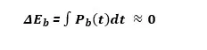
Fuel Consumption for a hybrid vehicle
is calculated as,
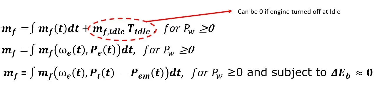
As seen, an extra power unit gives the ability to dynamically change the power operating point of the engine
In some cases, the engine, the engine power output might be higher than desired and in some lower, based on which point is more efficient, subject to keeping the net battery energy change 0.
This means, the local instantaneous fuel consumption minimization might not necessarily result in the global fuel consumption minimization. This makes hybrid vehicle complex, requiring the information of the entire trip beforehand to produce the most efficient control.
MATLAB Script for Initialization:
%% Skill-Lync -> Hybrid Drives Development
% Project 2 - Conventional Vehicle Model
% By - Ganeshram D
Simulink model of conventional vehicle:
In this project, a typical midsize car with a 1.9L engine and a 4-speed automatic transmission is considered and Honda Insight motor and battery are considered.
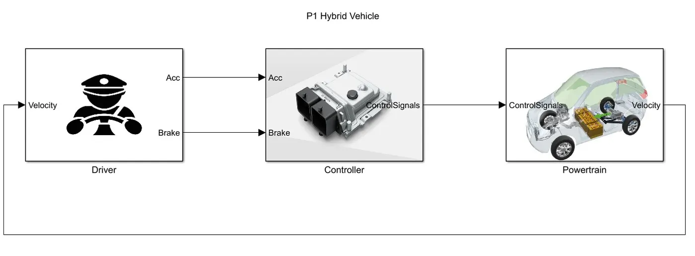
The Simulink model for the convection vehicle model having 3 main subsystems for the driver model, control model and powertrain block.
The actual vehicle speed is given as feedback to the driver block, and the driver block gives the controller block the required acceleration, torque, brake and power output, while the controller block provides control signals for engine torque, gear shifting and brake torque to the Powertrain model.
Driver Model:
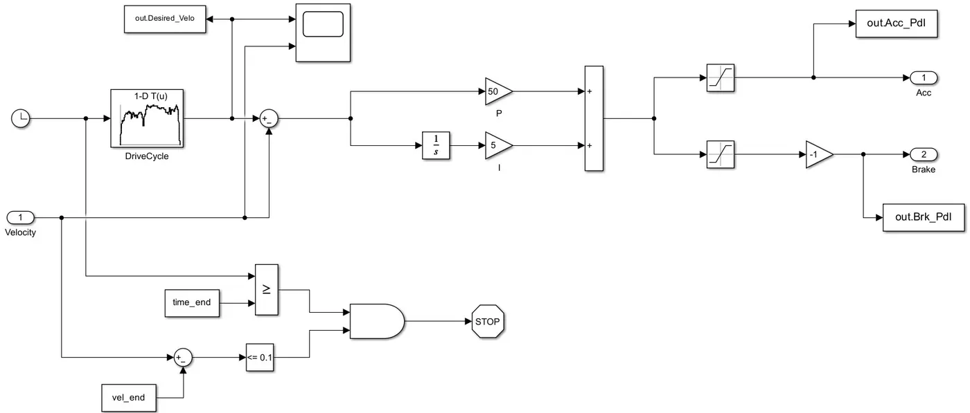
Driver Model is a basic PI controller that generates accelerator and brake pedal outputs to match the desired and actual vehicle speeds. The Proportional and integrator controls the error between desired output and actual speed through feedback controls
Controller Model:
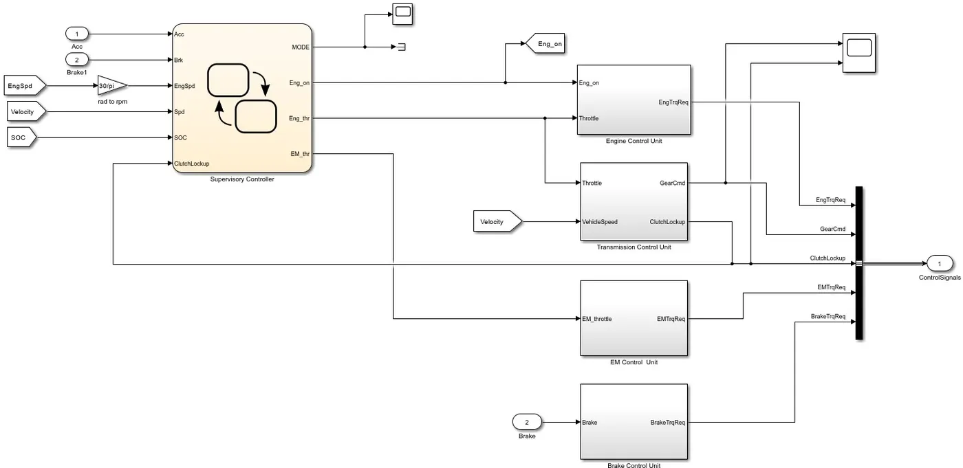
The controller takes in all the current conditions like acceleration, break, engine speed, SOC of battery, Velocity and the clutch lockup values and then analyses it and provide output to each controllers to perform as desired.
The Controller block has 4 controller : Engine control unit, Transmission Control unit, Electric Motor Control unit and the Brake Control unit.
All the control units are supervised or controlled by a Supervisory control unit.
Two scop blocks were used here to monitor the Mode shifting and Engine torque required, Gear command and Bake Torque required.
All the output of this block is fed to the 'bus creator' which will be fed to the power train as control signal.
Supervisory
Controller:
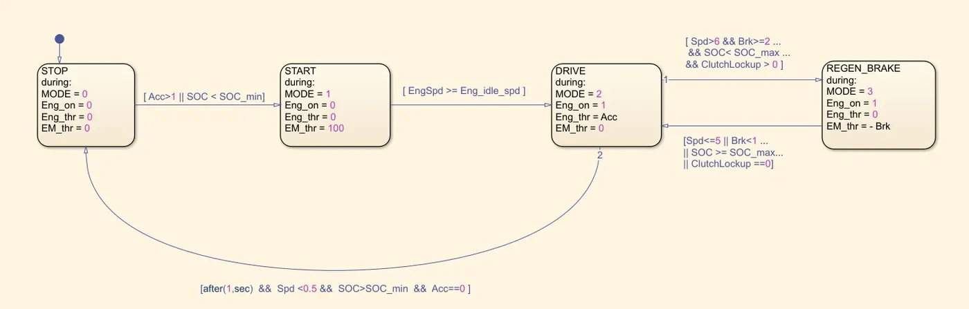
- The supervisory controller is modelled using State flow.
- The chart takes in Acceleration, Brake, Engine speed, SOC, Velocity, Clutch lockup values and depending on the conditions modelled inside the chart block it gives out the when all the engine should be kept on, what should be engine throttle and what should be the Electric motor throttle.
- The supervisory controller shifts between 4 modes: Stop, Start, Driving and Regeneration mode.
- It analyses and decide when to give the electric motor input and when to keep the engine on and off and when to do the regeneration while breaking.
Engine
Control Unit &
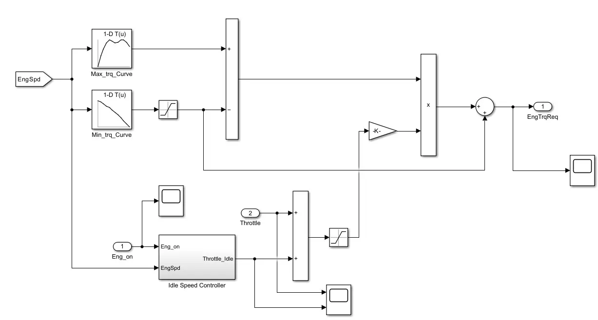
Engine Control Unit Compare engine speed with the maximum torque and minimum torque curves of the lookup table and give the required torque command to the engine block.
Idle Speed Controller:
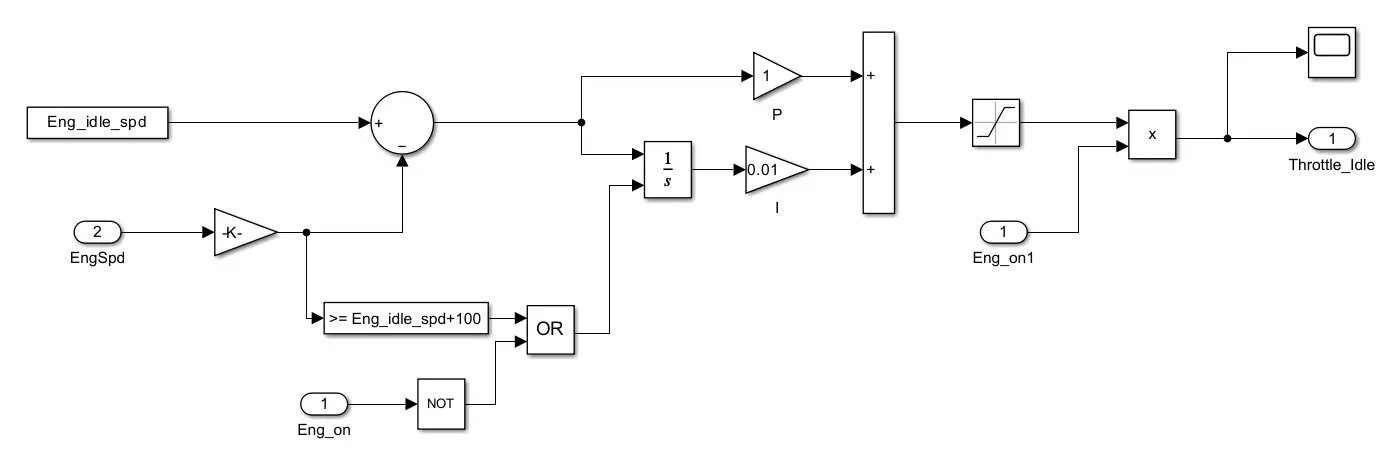
The throttle input is combined with the idle speed throttle and gains with the torque output from the lookup table to estimate the torque input required for the engine.
Transmission Control Block:
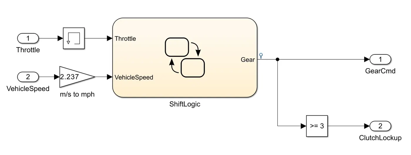
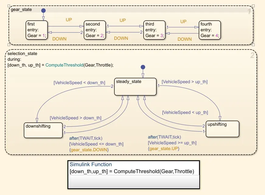
The transmission control block controls the gear shifting using the study flow Variable chart. The Gear shifting is Controlled according to the vehicle speed and throttle input. The gear command is passed to the Transmission block to select the desired gear ratio.
EM Control Unit –
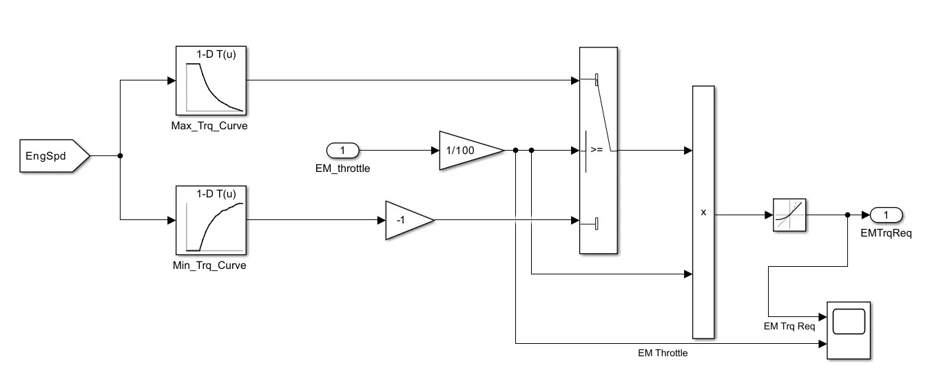
- EM control unit controls the torque required by the vehicle.
- The block takes in the throttle required by the vehicle which it get form the supervisory controller.
- Since the Electric motor is a P1 hybrid it is mounted directly on the crank shaft, the input of the motor is the engine speed itself.
- Using the lookup tables and the engine speed the model gives out the required torque which is to be generated by the electric motor.
Brake Control Unit:
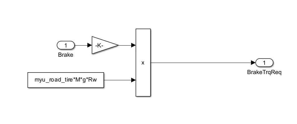
Brake Control unit Produce required brake torque according to the brake pedal input and passes the brake torque in to the wheel block in the transmission model.
Powertrain Model:
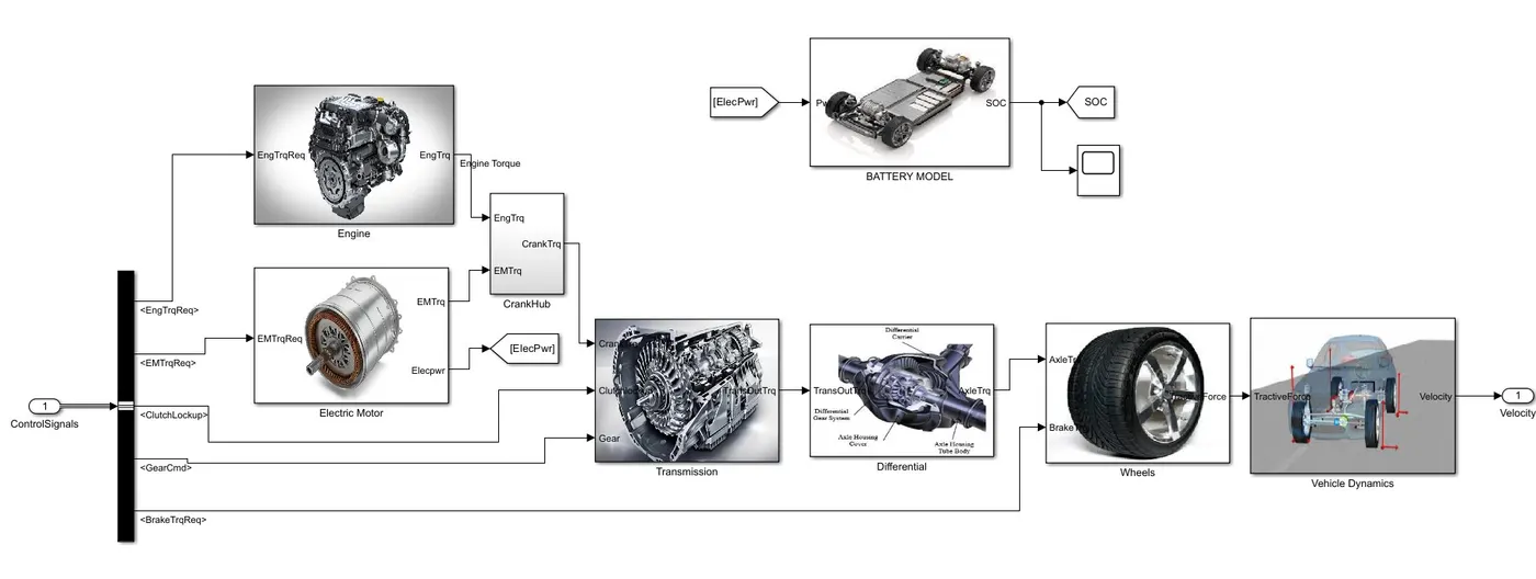
The powertrain model includes all the components that convert the power of the engine into vehicle motion. This includes Engine, Transmission, Electric Motor, Battery Differential, Wheels and the vehicle body dynamics subsystems.
 Engine
Model:
Engine
Model:
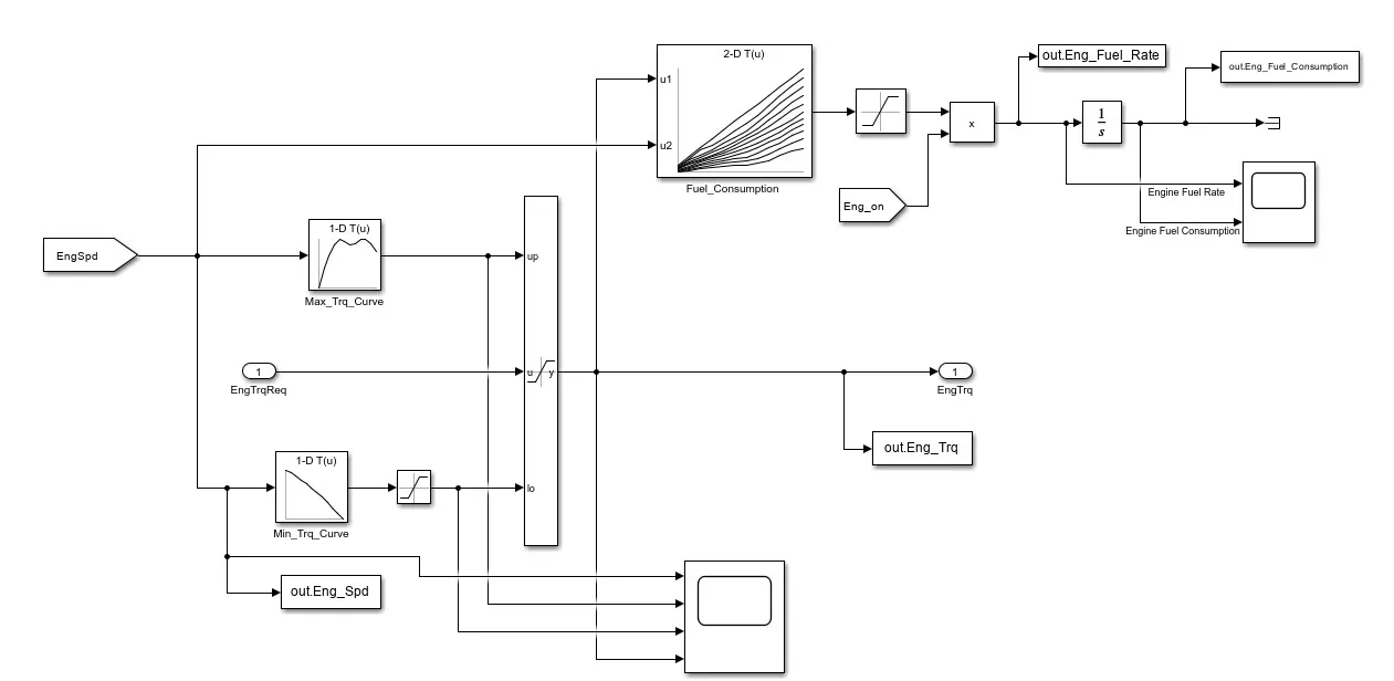
Based on the Engine speed The required torque from the controller is saturated between Max torque curve and min torque curve and passes the Engine torque to the Transmission block
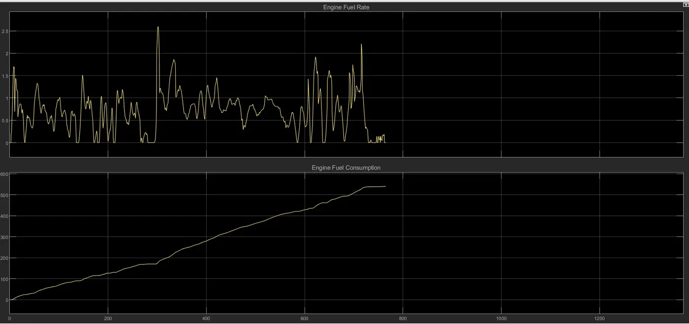
The 2D lookup table is used to calculate the fuel flow rate based on engine speed and engine torque. The fuel flow rate is then integrated to find the fuel consumption.
Estimated fuel flow rate, fuel consumption, engine torque and engine speed are passed to the MATLAB workspace using the to-workspace block.
Scope Results of Engine:
Transmission
Model:
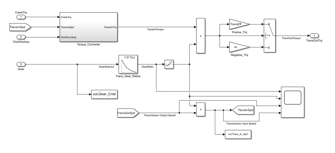
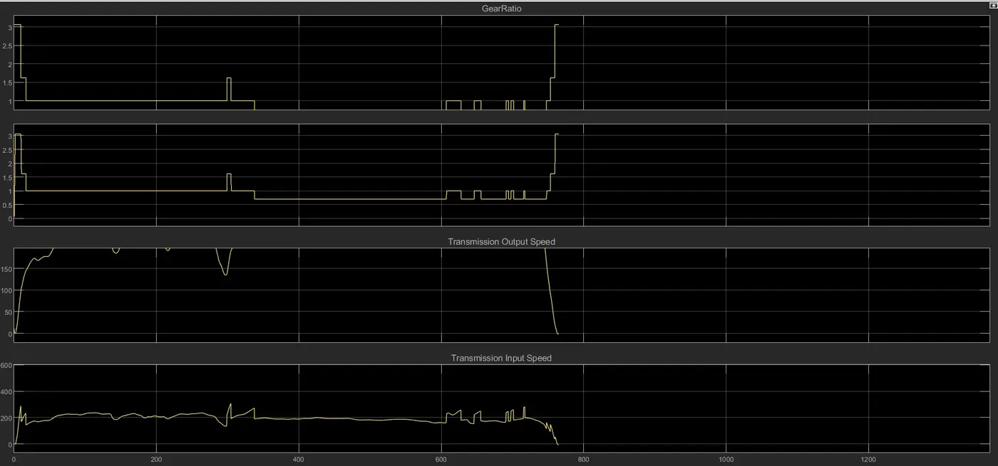
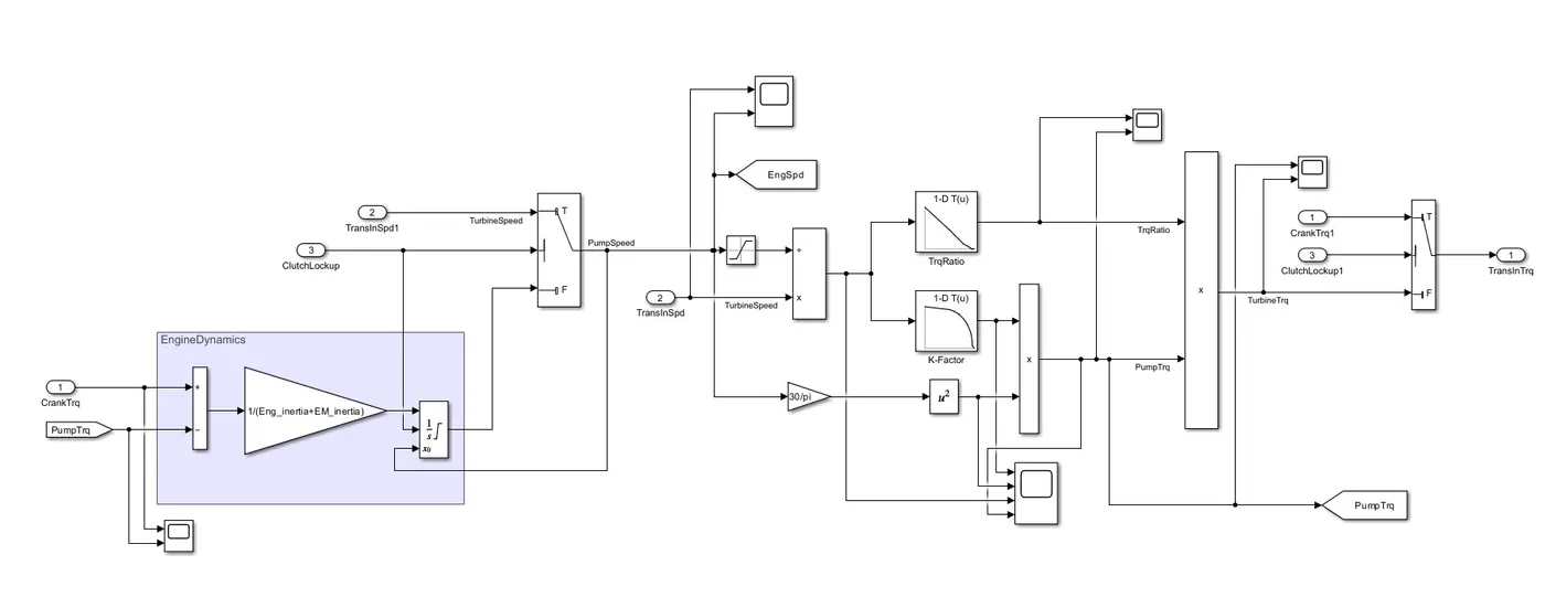
The engine block is connected to the automatic transmission via a torque converter. The output of the transmission is connected to the differential.
Scope Results of Transmission:
Torque Converter:
The gear selection from the transmission control unit is multiplied by the engine torque in this block, and the efficiency and engine dynamics of the torque converter are applied in this model.
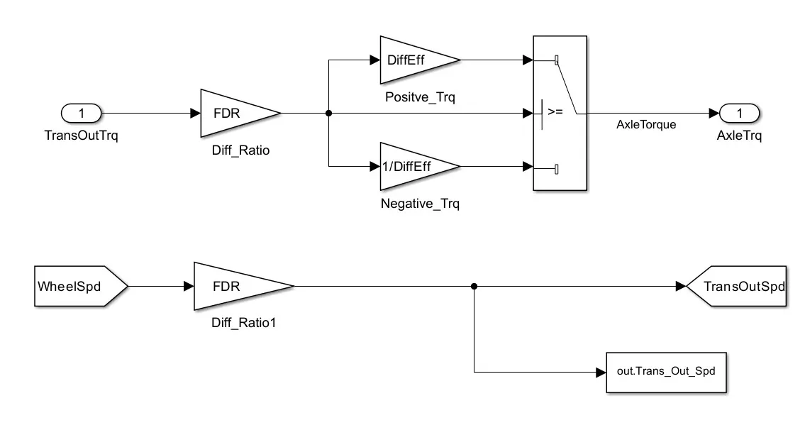
Differential Model:
The transmission output torque is multiplied by the differential ratio and differential efficiency in this block and the torque is transmitted to the wheel as the axle torque.
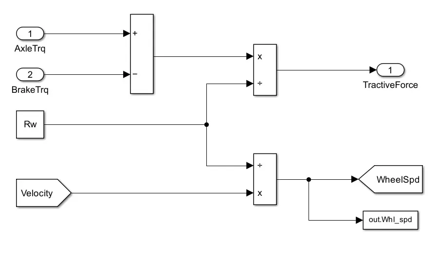
Wheel Model:
The brake torque from the control model is subtracted from the Axle torque and divides from the rolling radius to determine the Tractive force. The Wheel speed is calculated from the vehicle velocity.
 Electric
Motor:
Electric
Motor:
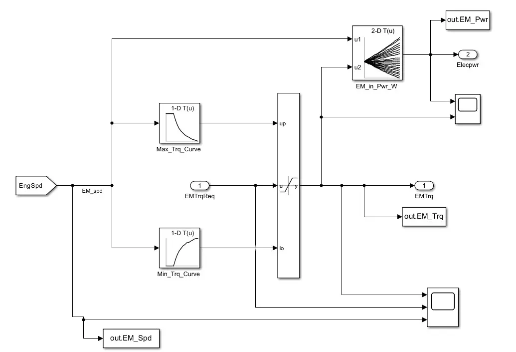
The Electric Motor take in the Torque requirement from the controller block and depending on the engine speed (which is the motor speed itself), it produces torque and power required.
The motor power is required to draw the power form the battery pack as the motor keeps on working.
This is done using speed - torque lookup tables.
Two scop blocks are used here one is to monitor the motor speed and the Motor torque required Torque given and the other to monitor the power drawn and the torque generated.
Crank Hub:
The crank hub takes in the engine torque and the electric motor torque and it adds up.
The crank torque is the sum of engine torque and the engine torque.
A
scope block is used to monitor the electric motor torque, engine torque and the
crank torque.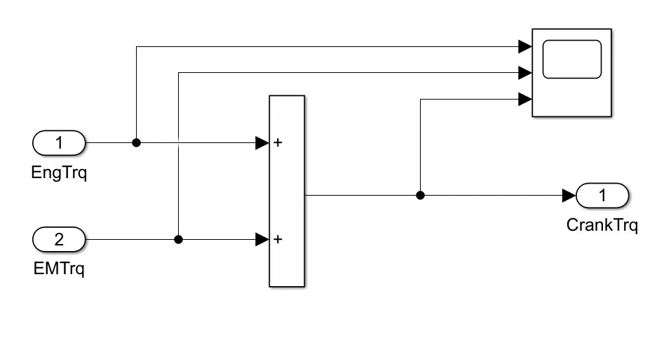
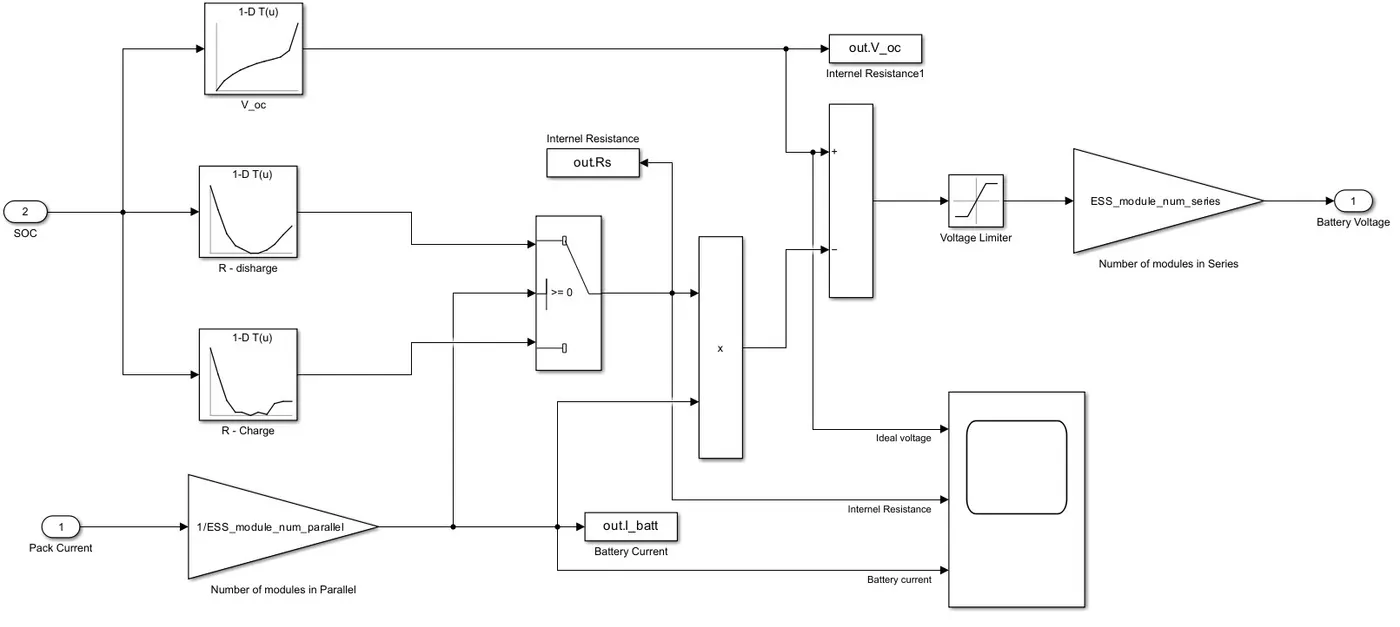
Energy Storage System (Battery):
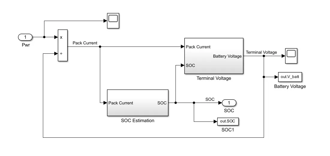
The ESS is the energy storage for the electric motor and is used to find the SOC and also the terminal voltage and pack current of the battery pack.
It takes in the Electric motor power used by the motor and also store the energy during regenerative braking.
The battery pack also has to maintain its state of charge whenever it goes below Charge sustaining mode in HEVs.
State of Charge (SOC) Model:
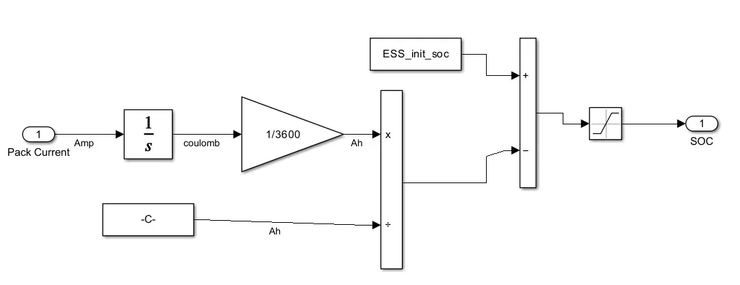
Dimensionless value that represents the amount of usable capacity remaining at a given time compared to the nominal battery capacity. Expressed in percentage of the rated capacity.
Terminal Voltage Model:
Vehicle Dynamics Model:
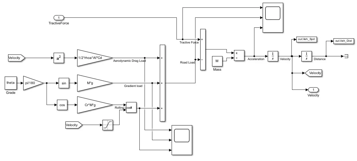
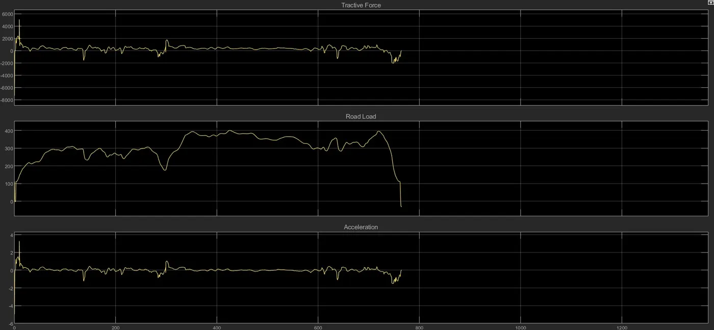
The longitudinal dynamics of the vehicle along with the road load is represented in the ‘Vehicle Dynamics’ block
Scope Results of Vehicle Dynamics:
Listing forces different applicable as per the scenario:
Tractive effort and resistance are the two main forces that oppose one another and determine the performance of roadway vehicles. Tractive effort is the force exerted against the roadway surface to allow a vehicle to move forward. Resistance encompasses all forces that push back and impede motion. Both of these are in units of force.

Rolling Resistance
Rolling resistance is caused by the interaction of tires with the roadway surface. Three main causes exist that create this resistance. The first is the rigidity of the tire and the roadway surface. The second is tire pressure and temperature. The third is vehicular operating speed.

Aerodynamic Resistance
Aerodynamic resistance is a force that is produced by turbulent air flow around the vehicle body. This turbulence is dependent on the shape of the vehicle, as well as the friction of air passing over the vehicle's surface. A small portion of this resistance comes from air flow through vehicle components, such as interior ventilation.

Grade Resistance
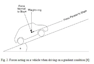
Grade resistance is the simplest form of resistance. It is the gravitational force acting on the vehicle. This force may not be exactly perpendicular to the roadway surface, especially in situations when a grade is present. Angle created between horizontal and the slope is θ. Several industrial vehicle manufacturers call the ability of the vehicle to run on a slope as Gradeability. Unit for gradeability is percent. Gradeability is calculated by multiplying tan θ with 100%.

Acceleration –
Inertia is force that inhibits the vehicle to reach a certain speed in a certain time. It is impossible for vehicle to achieve a certain speed from its idle position without acceleration. Therefore, to get to certain speed, the vehicle should be able to perform acceleration.

Power required at wheels is given by:
The power required at the wheels of a vehicle can be calculated using the formula P = Fv, where P is power, F is force, and v is velocity.

Post-Processing P1 Hybrid Vehicle in simulation model:
Output Results:
#1 Tabulate the fuel economy numbers (kmpl) for UDDS and HWFET cycle. This forms the baseline numbers for comparing with the conventional vehicle model.
UDDS Drive Cycle (Hybrid Vehicle) -

UDDS Drive Cycle (Conventional Vehicle) -

Comparisons of Hybrid and Conventional UDDS Cycle-
The fuel economy of the typical midsize car having a 1.9L engine and a 4-speed automatic transmission of Hybrid drive mode is higher (i.e. 1.1 kmpl) in the Urban driving condition compare to Conventional driving mode
HWFET Drive Cycle (Hybrid Vehicle) -

HWFET Drive Cycle (Conventional Vehicle) -

Comparisons of Hybrid and Conventional HWFET Drive Cycle-
The fuel economy of the typical midsize car having a 1.9L engine and a 4-speed automatic transmission of Hybrid drive mode is higher (i.e. 0.7 kmpl) in the Highway driving condition compare to Conventional driving mode
#1 Comments -
The fuel economy of the typical midsize car having a 1.9L engine and a 4-speed automatic transmission of Hybrid drive mode is higher in the highway driving condition compare to urban driving condition where frequent stoppage of vehicle can experience.
#2 Plot the time trace for engine, transmission input, transmission output and wheel speed
UDDS Drive Cycle -
HWFET Drive Cycle -
#2 Comments -
In UDDS drive cycle, Due to the frequent stoppage and idle loss, the input speed is facilitated by the torque converter and the transmission input speed fluctuates according to the engine torque required to achieve the drive cycle. But in Highway drive cycle, the speed flotation is comparatively less (almost nil) and no idle losses. Wheel speed and transmission output speed vary according to gear and differential ratio.
#3 Plot engine torque, engine power, fuel rate and fuel consumption:
UDDS Drive Cycle -
HWFET Drive Cycle -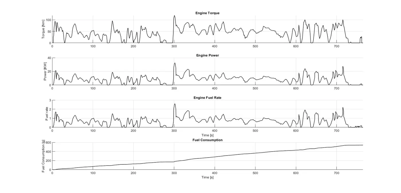
#3 Comments -
In UDDS drive cycle, Due to the frequent stoppage and idle loss, torque, Power requirements are less compared to the HWFET drive cycle which has high torque and power requirements
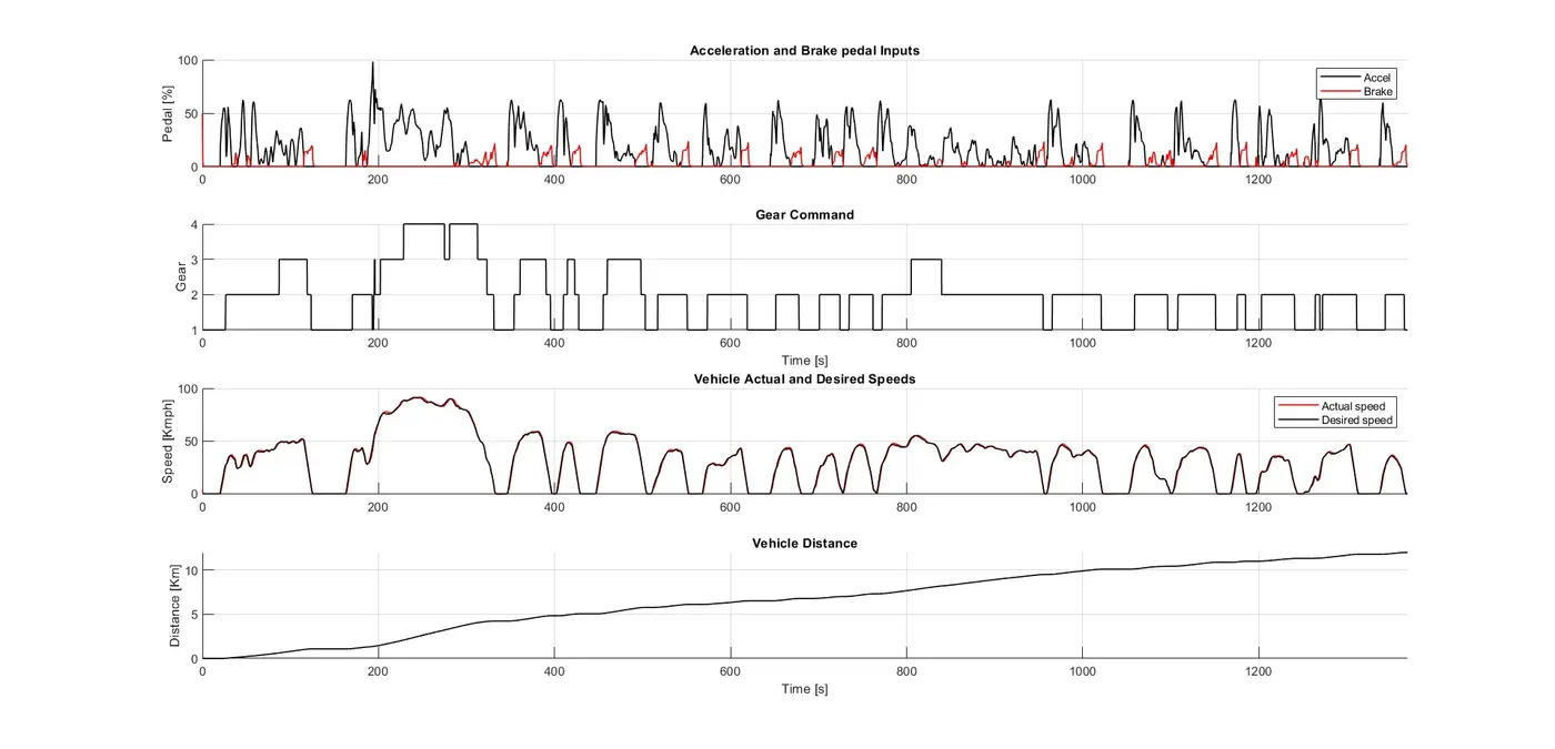
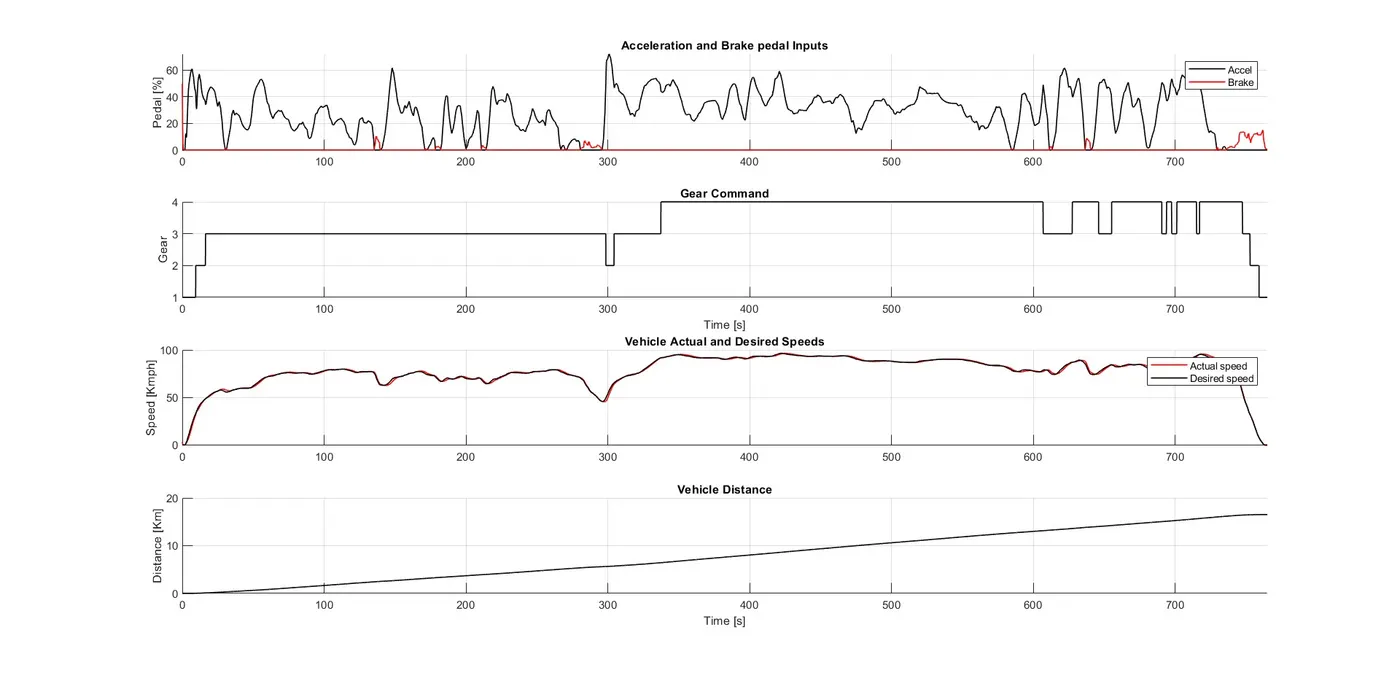
#4 Plot accelerator and brake pedal, gear command, vehicle desired and actual speed, vehicle distance
UDDS Drive Cycle -
HWFET Drive Cycle -
 #4
Comments –
#4
Comments –
In UDDS Drive cycle, Brake requirements are higher, less accelerator pedals and gear shifts often occur because this drive cycle is running with fluctuating speed, but in HWFET drive cycle Brake requirements are lower, more accelerator pedals are applied on the highway drive cycle, and gear shifts often occur because the drive cycle is smoother
#5 Plot the engine operating points on the engine fuel map
UDDS Drive
Cycle -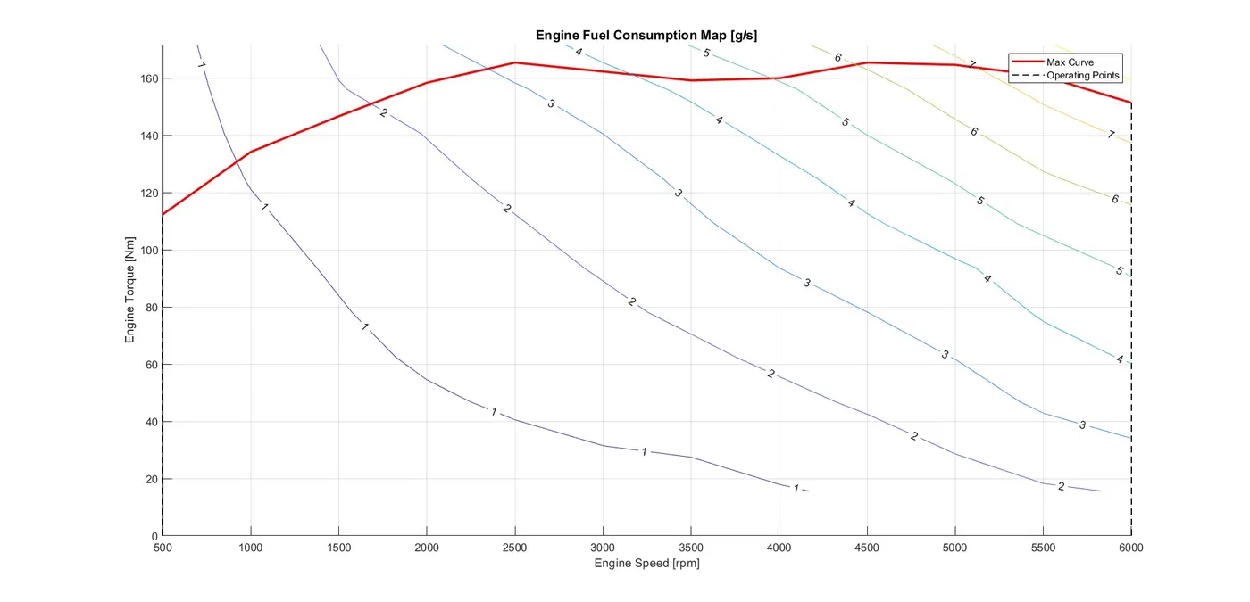
HWFET Drive Cycle -
#5 Comments -
In
UDDS & HWFET Drive cycle, we can see the maximum operating speed of the engine is
between 500 RPM and 6000 RPM and similarly the maximum torque (165Nm) is achieved at 2500 to 4500 RPM range.
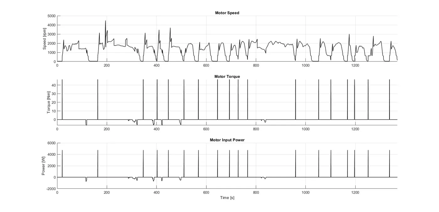
#6 Plot
motor speed, torque, motor input power using subplots.
UDDS Drive Cycle -
HWFET Drive Cycle -
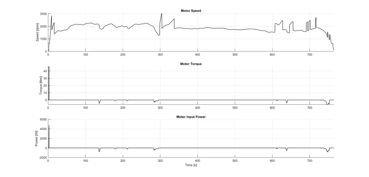
#6 Comments -
In UDDS drive cycle due to frequent stoppage, when vehicle accelerating the torque,power requirement is more when the motor acts as a starter motor & In HWFET Drive cycle, the torque,power requirements is less compare to Urban cycle
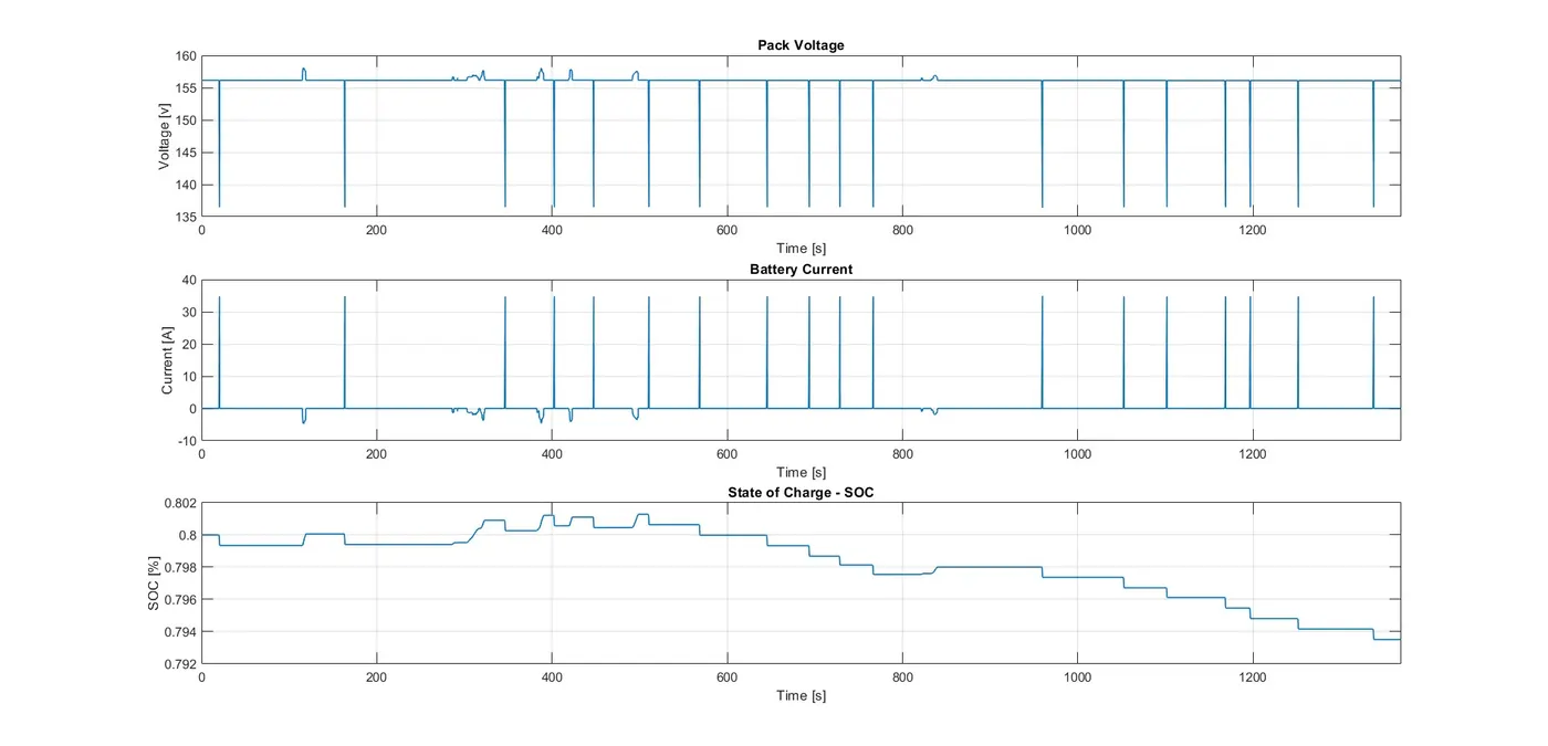
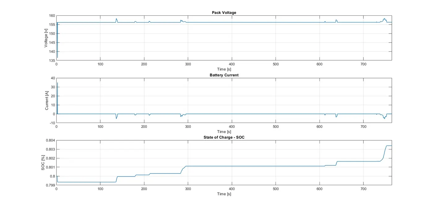
#7 Plot pack voltage, current and SoC using subplots.
UDDS Drive Cycle -
HWFET Drive Cycle -
#7 Comments -
In UDDS the SOC was gradually decreasing, but in HWFET the SOC went down quickly and then stated to gain charge.
This shows that the regen is high in HWFET and the other reason is that there is very less gear shifting and braking.
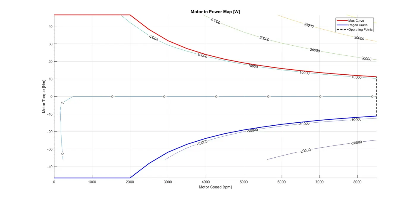
#8 Plot the motor operating points on the motor input power map, with the motor max motoring and generating torque curves.
UDDS Drive Cycle -
HWFET Drive Cycle -
#8 Comments -
From the graph we can find that the motor operating point is the speed between 0 rpm and 8500 rpm which is bounded by the max torque while motoring which is 46 Nm and generating torque curve which is also 46 Nm.
#9 Generate the plots for both drive cycles
UDDS Drive
Cycle -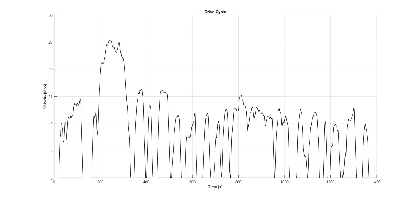
HWFET Drive Cycle -
#9 Comments -
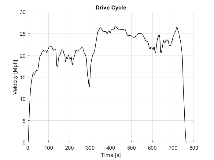
In UDDS drive cycle, velocity/speed of the vehicle is fluctuating over the time due to running in urban roads where the frequent stoppage and idle losses are more compare to High drive cycle.
In HWFET drive cycle, velocity/speed of the vehicle is comparatively less (almost nil) and no idle losses. Hence the distance covered by the high way driven condition vehicle is more compare to urban driven condition driven
Conclusion:
- The forward energy-based fuel consumption model of a P1 Hybrid Vehicle has been successfully Simulated using MATLAB and Simulink.