Project 2
Project Aim :
Create a MATLAB model of an electric car that uses a lithium-ion battery and a suitable motor. Choose suitable blocks from Simscape or Powertrain block set. Implement the vehicle speed control using a PI controller and generate brake and accelerator commands. Avoid using a ready-made driver block for speed control.
Prepare a report about your model including the following:
Objectives, System-level configurations, Model parameters, Results, Conclusion.
(Note- The Simulink model file should be compulsorily attached)
Objectives:
- To make the simple and low run-time vehicle model using the individual component model.
- Implementation of a PI controller to generate brake and accelerator commands for the vehicle.
- To check out performance parameters: Speed, SOC, current, the temperature of motor and H-bridge, etc. with various drive cycles.
- To Obtain the results with three different drive cycles are FTP, WOT, and 45 km/hr constant speed for 100Km distance.
- To experiment with Motor power, vehicle body (Rolling resistance, Air drag, weight) inputs and understand the key factors behind the model output dependencies.
- To know the MATLAB model and its configuration to match with an actual small electric vehicle.
Answer:
An electric vehicle (EV) is a vehicle that uses one or more electric motors or traction motors for propulsion. An electric vehicle may be powered through a collector system by electricity from off-vehicle sources, or may be self-contained with a battery, solar panels, fuel cells or an electric generator to convert fuel to electricity. EVs include, but are not limited to, road and rail vehicles, surface and underwater vessels, electric aircraft and electric spacecraft.
EVs first came into existence in the mid-19th century, when electricity was among the preferred methods for motor vehicle propulsion, providing a level of comfort and ease of operation that could not be achieved by the gasoline cars of the time. Modern internal combustion engines have been the dominant propulsion method for motor vehicles for almost 100 years, but electric power has remained commonplace in other vehicle types, such as trains and smaller vehicles of all types.
Commonly, the term EV is used to refer to an electric car. In the 21st century, EVs have seen a resurgence due to technological developments, and an increased focus on renewable energy and the potential reduction of transportation's impact on climate change and other environmental issues. Project Drawdown describes electric vehicles as one of the 100 best contemporary solutions for addressing climate change.
Government incentives to increase adoption were first introduced in the late 2000s, including in the United States and the European Union, leading to a growing market for the vehicles in the 2010s. Increasing public interest and awareness and structural incentives, such as those being built into the green recovery from the COVID-19 pandemic, is expected to greatly increase the electric vehicle market. A pre-COVID 2019[when?] analysis projected that Electric vehicles are expected to increase from 2% of global share in 2016 to 22% in 2030. Much of this market growth is expected in markets like North America and Europe; a 2020 literature review suggested that growth in use of electric vehicles, especially electric personal vehicles, currently appears economically unlikely in developing economies.
Here, a small electric vehicle model is referred from reference no. 1, and a Simulink model is developed based on its parameters up to some extent, which is the e-kuv 100 of Mahindra company.
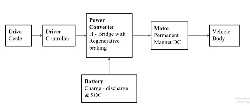
In this project, the parameters of the referred a small electric vehicle are considered and the goal is to make it as much realistic as it can be, considering the limitations of a simple and low-runtime model of the same time. In the following literature, we will first give brief descriptions about each of the blocks used in Simulink, and the parameters being considered and given to the model will also be discussed and shown during the same. After that, all Input-Outputs results will be given as per the requirement. The following Screenshot gives us an idea of what parameter values are employed here to develop the electric vehicle model.
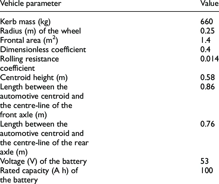
However, the rating of the battery and the motor is increased to have a more realistic responses from the output side. Rest of the things remains the same.
(A) Individual Block Representations:
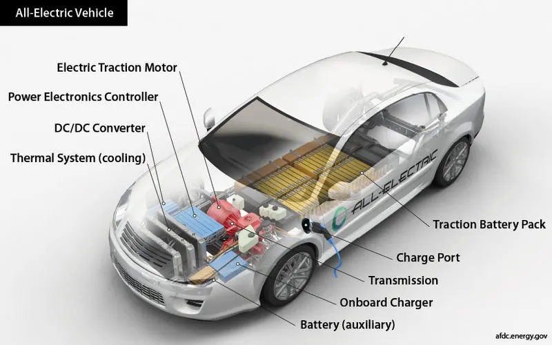
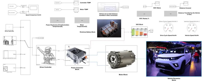
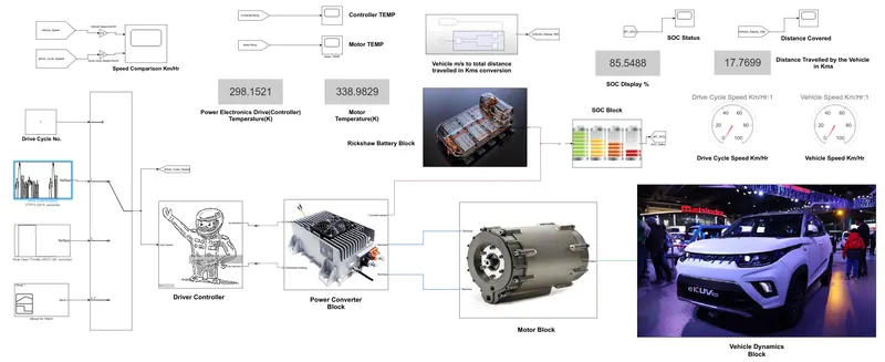
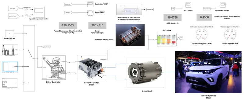
The entire Simulink model can be divided into main 5 blocks which are there. Each of them is described briefly one after the other in the following sections. In the designed Electric Rickshaw main blocks is Battery, drive cycle, controller, DC Motor, Vehicle body & Transmission system. Drive cycle is the input data like how a human drives his actual vehicle here FTP75, WOT & Excel (Manually Prepared in Excel sheet) drive cycles are used to make the designed vehicle to give the output how it reacts to the drive cycle. The main objective is to obtain the speed by the driver, to estimate the temperature of the Motor and Controller, to estimate the sates of charge (SOC), distance traveled by the vehicle. There is a SOC block that will estimate the state of charge of a battery, distance is calculated by speed and time parameters for all three Drive cycles.
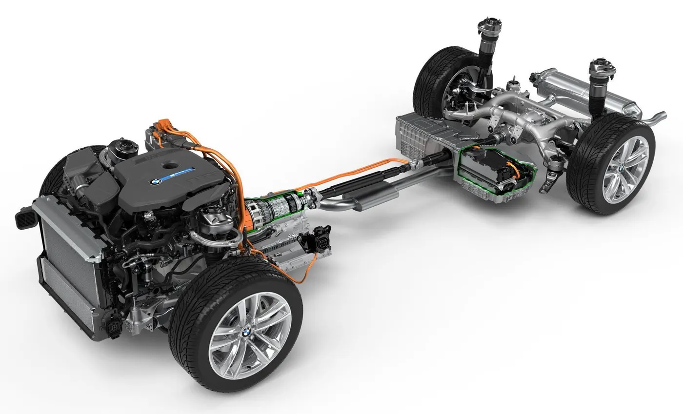
Drive-train of an Electric Vehicle
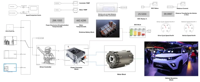
The main Simulink model for the small electric vehicle as a whole, is represented like the following diagram is shown:
(1) Vehicle Dynamics Block:
A general conceptual image of electrical vehicle dynamics
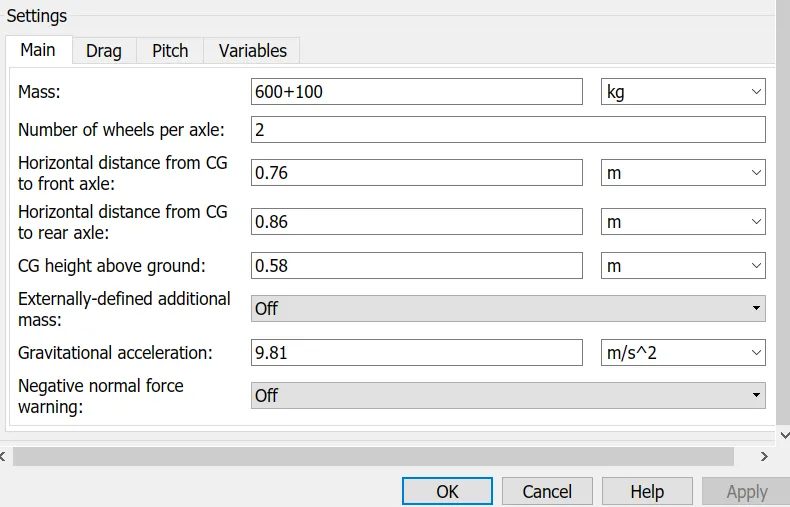
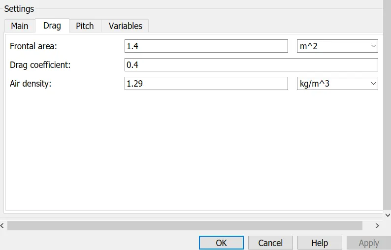
This block consists of 4 wheel tire systems, represents a two-axle vehicle body in longitudinal motion. The block accounts for body mass, aerodynamic drag, road incline, wind speed, and weight distribution between axles due to acceleration and road profile. The vehicle can have the same or a different number of wheels on each axle. It can optionally include pitch and suspension dynamics or additional variable mass and inertia. The vehicle does not move vertically relative to the ground and it is where all the vehicle body-related parameters are given, to match the dynamics with the referred one.
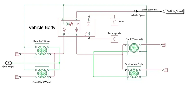
Connection H is the mechanical translational conserving port associated with the horizontal motion of the vehicle body. The resulting traction motion developed by tires should be connected to this port. Connections V, NF, and NR are physical signal output ports for vehicle velocity and front and rear normal wheel forces, respectively. Wheel forces are considered positive if acting downwards. Connections W and beta are physical signal input ports corresponding to headwind speed and road inclination angle, respectively. If the variable mass is modeled, the physical signal input ports CG and M are exposed. CG accepts a two-element vector representing the x and y distance offsets from vehicle CG to additional load mass CG. M represents the additional mass. If both variable mass and pitch dynamics are included, the physical signal port J accepts the inertia of the additional mass about its own CG.
----------------------------------------------
The Tire Magic Formula represents the longitudinal behavior of a highway tire characterization. The block is built from Tire-Road Interaction (Magic Formula) and Simscape Foundation Library Wheel and Axle blocks. Optionally, the effects of tire inertia, stiffness, and damping can be included.
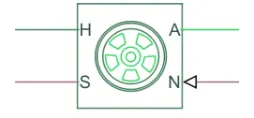
Connection A is the mechanical rotational conserving port for the wheel axle. Connection H is the mechanical translational conserving port for the wheel hub through which the thrust developed by the tire is applied to the vehicle. Connection N is a physical signal input port that applies the normal force acting on the tire. The force is considered positive if it acts downwards. Connection S is a physical signal output port that reports the tire slip. Optionally expose physical signal port M by setting Parameterize by to Physical signal Magic Formula coefficients. Physical signal port M accepts a four-element vector corresponding to the B, C, D, and E Magic Formula coefficients.
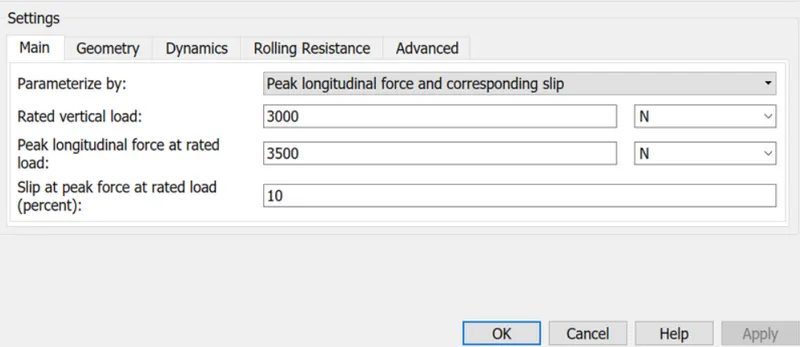
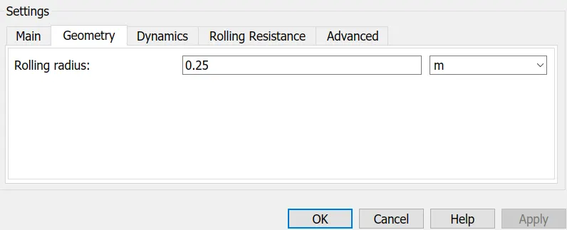
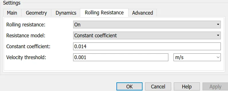
(2) Motor Block:
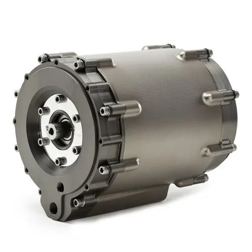
The motor block consists of a permanent magnet DC motor, Gear-Ratio box, inertia component for the motor mechanical part, and the temperature sensor to measure the temperature of the PMDC motor throughout its operation.
The block assumes that no electromagnetic energy is lost, and hence the back-emf and torque constants have the same numerical value when in SI units. Motor parameters can either be specified directly or derived from the no-load speed and stall torque. If no information is available on armature inductance, this parameter can be set to some small non-zero value.
When a positive current flows from the electrical + to - ports, a positive torque acts from the mechanical C to R ports. Motor torque direction can be changed by altering the sign of the back-emf or torque constants. PS to Simulink converter is used for taking the temperature output to Simulink library variable. The thermal inputs of the motor are also given as per the referred parameters.
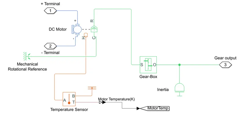
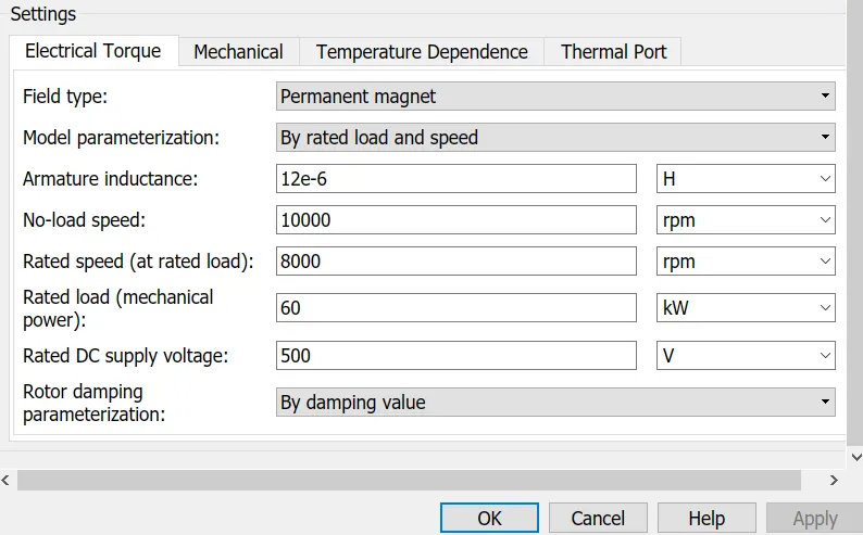
The parameter inputs are given below for each block that is part of this block.
DC Motor -->
This block represents the electrical and torque characteristics of a DC motor. The block assumes that no electromagnetic energy is lost, and hence the back-emf and torque constants have the same numerical value when in SI units. Motor parameters can either be specified directly or derived from the no-load speed and stall torque. If no information is available on armature inductance, this parameter can be set to some small non-zero value.
When a positive current flows from the electrical + to - ports, a positive torque acts from the mechanical C to R ports. Motor torque direction can be changed by altering the sign of the back-emf or torque constants.
-------------------------------------------------------
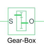
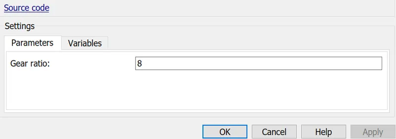
The block represents an ideal, non-planetary, fixed gear ratio gearbox. The gearbox is characterized by its only parameter, Gear ratio, which can be positive or negative. Connections S and O are mechanical rotational conserving ports associated with the box input and output shaft, respectively. The gear ratio is determined as the ratio of the input shaft angular velocity to that of the output shaft. The block generates torque in a positive direction if a positive torque is applied to the input shaft and the ratio is assigned a positive value.
------------------------------------
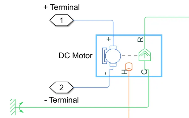
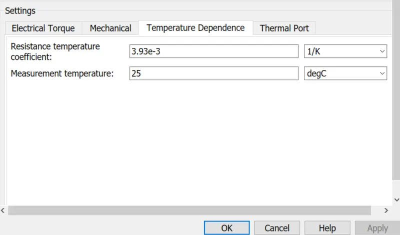
The DC Motor has an optional thermal port, hidden by default. To enable the thermal port, just right-click the block in your model, and then from the context menu select Simscape --> Block choices --> Show thermal port.
This action displays the thermal port H on the block icon (given in the DC motor figure) and exposes the Temperature Dependence and Thermal Port parameters.
Use the thermal port to simulate the effects of copper resistance losses that convert electrical power to heat. For more information on using thermal ports and on the Temperature Dependence and Thermal Port parameter.
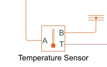
This block measures temperature in a thermal network. There is no heat flow through the sensor. The physical signal port T reports the temperature difference across the sensor. The measurement is positive when the temperature at port A is greater than the temperature at port B.
(3) Power Converter Block:
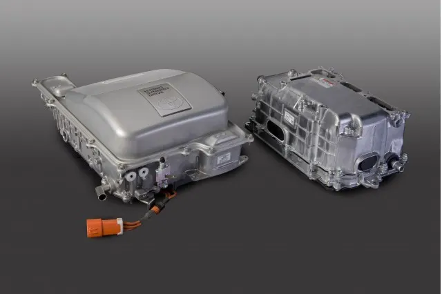
This block consists of controlled PWM voltage, H-bridge, current sensor, and temperature sensor. The thermal port of the H-bridge is enabled from the simscape options to measure its temperature throughout the operation using a temperature sensor block.
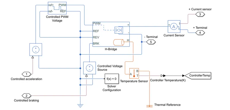
--------------------------------------------------------
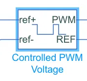
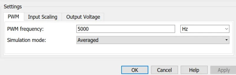
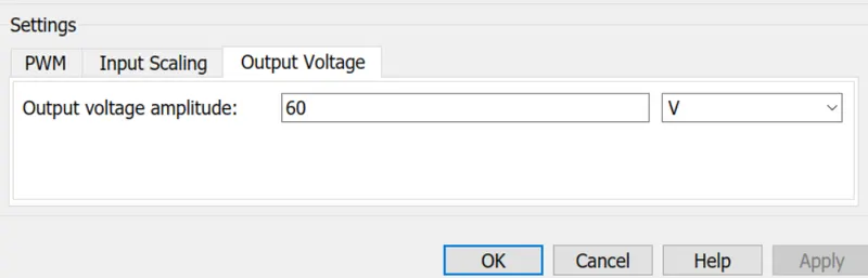
This block creates a Pulse-Width Modulated (PWM) voltage across the PWM and REF ports. The output voltage is zero when the pulse is low and is equal to the Output voltage amplitude parameter when high. The duty cycle is set by the input value. Right-click the block and select Simscape--->Block choices to switch between electrical +ref/-ref ports and PS input u to specify the input value. At time zero, the pulse is initialized as high unless the duty cycle is set to zero or the Pulse delay time is greater than zero.
The Simulation mode can be set to PWM or Averaged. In PWM mode, the output is a PWM signal. In Averaged mode, the output is constant with a value equal to the averaged PWM signal.
Electrical input ports — The block calculates the duty cycle based on the reference voltage across its ref+ and ref- ports. This modeling variant is the default.
PS input — Specify the duty cycle value directly by using an input physical signal port.
Following parameters used in Controlled PWM voltage:
----------------------------------------
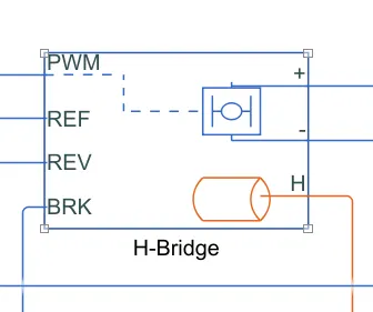
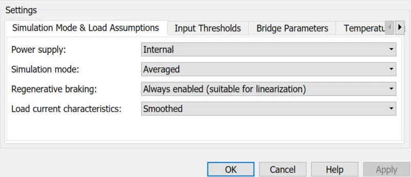
This block represents an H-bridge motor drive. The block can be driven by the Controlled PWM Voltage block in PWM or Averaged mode. In PWM mode, the motor is powered if the PWM port voltage is above the Enable threshold voltage. In Averaged mode, the PWM port voltage divided by the PWM signal amplitude parameter defines the ratio of the on-time to the PWM period. Using this ratio and assumptions about the load, the block applies an average voltage to the load that achieves the correct average load current. The Simulation mode parameter value must be the same for the Controlled PWM Voltage and H-Bridge blocks.
If the REV port voltage is greater than the Reverse threshold voltage, then the output voltage polarity is reversed. If the BRK port voltage is greater than the Braking threshold voltage, then the output terminals are short-circuited via one bridge arm in series with the parallel combination of a second bridge arm and a freewheeling diode. Voltages at ports PWM, REV, and BRK are defined relative to the REF port. If exposing the power supply connections, the block only supports PWM mode.
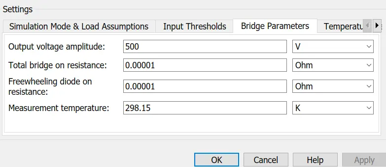
Electrical input ports — The block calculates the duty cycle based on the reference voltage across its ref+ and ref- ports. This modeling variant is the default.
PS input — Specify the duty cycle value directly by using an input physical signal port.
Following parameters used in Controlled PWM voltage:
-----------------------------------------------
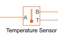
This block measures temperature in a thermal network. There is no heat flow through the sensor. The physical signal port T reports the temperature difference across the sensor. The measurement is positive when the temperature at port A is greater than the temperature at port B.
When the thermal port is visible in the H-bridge block--->
-
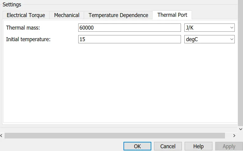
The heat generated by the bridge on-resistance and freewheeling diodes is added to the thermal port. The thermal port has an associated thermal mass and initial temperature that can be preset from the Thermal Port parameters.
-
The bridge on-resistance and freewheeling diode resistance become functions of temperature. You can define the values for these resistances and the second measurement temperature from the Temperature Dependence parameters. Resistance is assumed to vary linearly between the two measurement temperatures. Extrapolation is used for temperatures outside of this range, except for when simulating in averaged mode with discontinuous load current characteristics.
(4) Driver Controller Block:
The driver controller block is responsible for giving the acceleration input and deceleration input according to the input drive cycle. Even with all the parameters and other factors are perfect, if this controller block fails then it will not give the desired acceleration and deceleration inputs to the Electrical Drive System and then the vehicle will fail to follow the drive cycle. So, by this, we have a clear idea that how important the block is and it needs to be work perfectly to have our desired vehicle tracking outputs.
Now, to achieve good control over these inputs, we have to have correct values for any controller parameter gains to get the desired response. The controller can be PI, PID and it can be represented in many ways. For this process to employ the controller the PI controller Method is chosen as per the objectives.
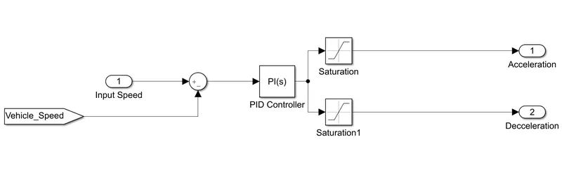
Proportional control, in engineering and process control, is a type of linear feedback control system in which a correction is applied to the controlled variable which is proportional to the difference between the desired value (setpoint, SP) and the measured value (process variable, PV). Two classic mechanical examples are the toilet bowl float proportioning valve and the fly-ball governor.
The proportional control concept is more complex than an on–off control system like a bi-metallic domestic thermostat, but simpler than a proportional–integral–derivative (PID) control system used in something like an automobile cruise control. On–off control will work where the overall system has a relatively long response time, but can result in instability if the system being controlled has a rapid response time. Proportional control overcomes this by modulating the output to the controlling device, such as a control valve at a level which avoids instability, but applies correction as fast as practicable by applying the optimum quantity of proportional gain.
A drawback of proportional control is that it cannot eliminate the residual SP − PV error in processes with compensation e.g. temperature control, as it requires an error to generate a proportional output. To overcome this the PI controller was devised, which uses a proportional term (P) to remove the gross error, and an integral term (I) to eliminate the residual offset error by integrating the error over time to produce an "I" component for the controller output.
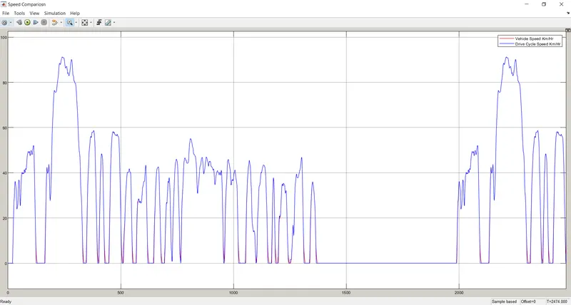
In this context, 3 different PI gain values were chosen manually and simulated with the FTP75 drive cycle to find out the results of each one of them and the best was is chosen at the end. The results are followed:
(i)P=3, I=1:
(ii)P=2, I=5:
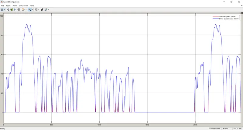
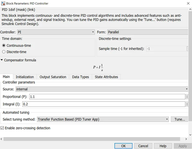
(iii)P=1.1, I=0.2:
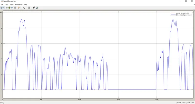
From the (iii) no experiment the PI is so well tuned that it coincides with the drive cycle data in the graph. Hence, the chosen PI parameter gains are: P=1.1 & I=0.2.
(5) Battery Block:
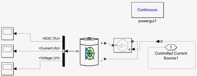
The battery is required to power the controller and motor. The controller uses the battery power according to produce the input given by the motor to obtain maximum speed. The battery is also used to power every electrical component in the vehicle. The battery has two-stage one is charging and another one is discharging state.
The Nominal voltage of the battery is 500 V
Initial SoC is 100%
The battery as a series internal resistance plus a charge-dependent voltage source defined by:
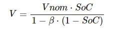
where SoC is the state of charge and Vnom is the nominal voltage. Coefficient beta is calculated to satisfy a user-defined data point [AH1, V1].
The battery has a positive and negative terminal which is given the voltage-controlled source where the battery consumption is controlled by the motor controller and then it is given to the SOC block. The battery parameters are given below:
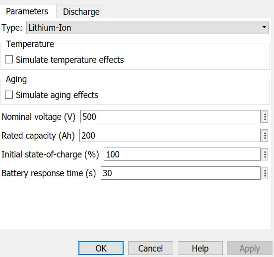
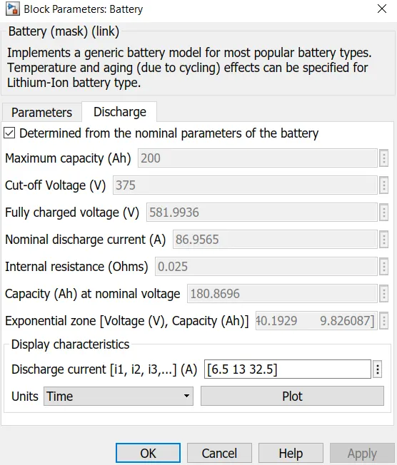
(6) Battery Current To SOC Conversion Block:
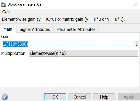
SoC is the percentage or level of battery present after certain travel or consumption of battery charge by the vehicle. In the designed vehicle battery charge or SOC is calculated by giving it to the rate transition and then to gain were 1/(nominal battery capacity); then to a discrete-time integrator and it will get minus from the 1 as it is considered a 100% of battery and it is multiplied with 100 to get a percentage of battery.
The majority of blocks are simscape blocks where physical to Simulink converter is used to convert the physical signal from simscape block to Simulink signal.
The SoC block is represented in the model like the following:
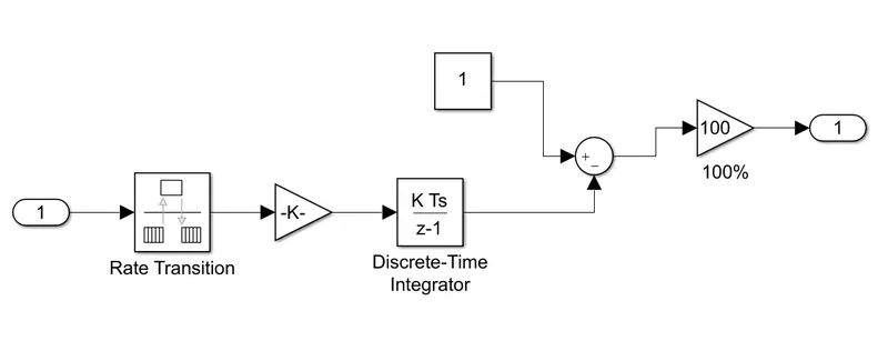
Just like the above, the current from the battery is fed to the rate transition block and to a gain block where the discharge rate is given and then it is fed to the discrete-time integrator. After that to make it in % SoC the rest of the block is arranged.
(7) Speed To Kms Conversion Block:
To measure the distance covered by the vehicle, its speed is being converted to the total distance covered by the vehicle i.e from m/s to Kms. The block is given below:
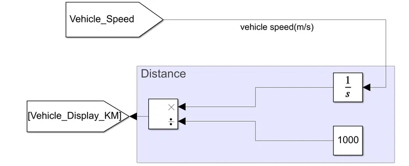
Here, from m/s it is come out in distance covered in meters when fed through the integrator block, and then diving it by 1000 gives us the distance covered in Kms.
(B) Input To The Simulink Model:
Total three drive cycles are chosen for this Simulink model and each time only one of the drive cycles is run as the input drive cycle. The three drive cycles are FTP, WOT, and a custom cycle which allows the rickshaw to run for a total distance of 100 Kms, with a constant speed of 45 Km/hr.
(1) FTP75 Urban Drive Cycle:
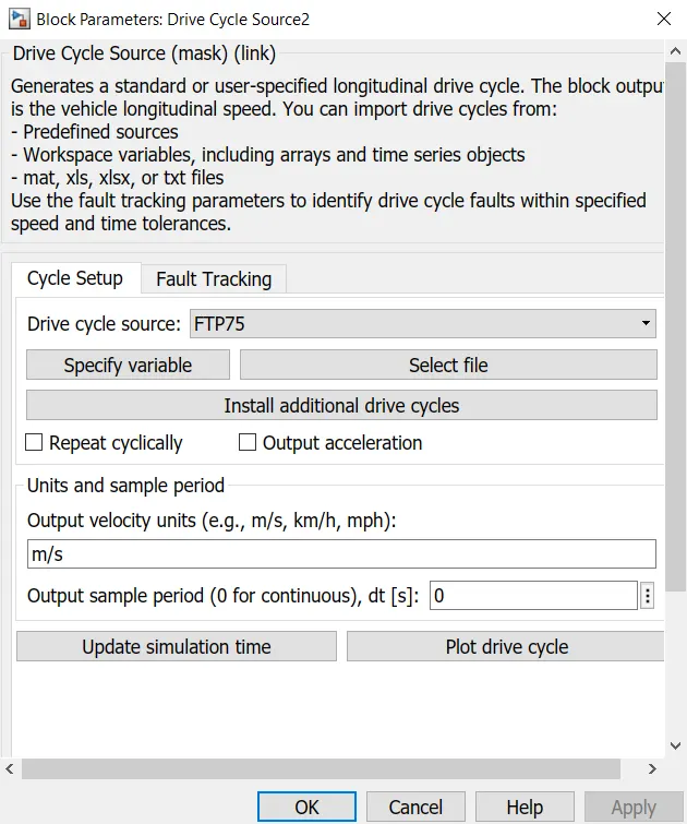
This Drive Cycle Source generates a standard or user-specified longitudinal drive cycle. The block output is the vehicle's longitudinal speed. You can import drive cycles from:
- Predefined sources
- Workspace variables, including arrays and time series objects
- mat, Xls, Xlsx, or txt files
Use the fault tracking parameters to identify drive cycle faults within the specified speed and time tolerances.
However, for this Simulink model, the standard FTP75 Drive Cycle is chosen.
The "city" driving program of the EPA Federal Test Procedure is identical to the UDDS plus the first 505 seconds of an additional UDDS cycle.
Then the characteristics of the cycle are:
- Distance traveled: 17.77 km (11.04 miles)
- Duration: 1874 seconds
- Average speed: 34.1 km/h (21.2 mph)
The procedure is updated by adding the "hot start" cycle that repeats the "cold start" cycle of the beginning of the UDDS cycle. The average speed is thus different but the maximum speed remains the same as in the UDDS. The weighting factors are 0.43 for the cold start and transient phases together and 0.57 for the hot start phase.
Though it was created as a reference point for fossil-fuelled vehicles, the UDDS and thus the FTP-75, are also used to estimate the range in distance traveled by an electric vehicle in a single charge.
(2) WOT Drive Cycle:
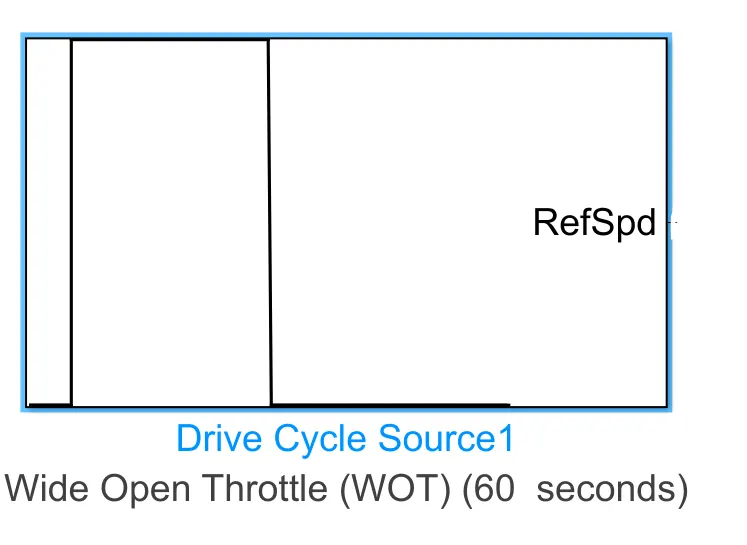
With the same drive cycle source block, the Wide Open Throttle or WOT is chosen instead of the FTP75 drive cycle.
Wide-open throttle or wide-open throttle (WOT), also called full throttle, is the fully opened state of throttle on an engine (internal combustion engine or steam engine). The term also, by extension, usually refers to the maximum-speed state of running the engine, as the normal result of a fully opened throttle plate/butterfly valve. In an internal combustion engine, this state entails the maximum intake of air and fuel that occurs when the throttle plates inside the carburetor or throttle body are "wide open" (fully opened up), providing the least resistance to the incoming air. In the case of an automobile, WOT is when the accelerator is depressed fully, sometimes referred to as "flooring it" (because automotive throttle controls are usually a pedal, so the full throttle is selected by pressing the pedal to the floor, or as near as it will go). A throttle on a steam engine controls how much steam is sent to the cylinders from the boiler.
In the case of a diesel engine, which does not have a throttle valve, WOT is the point at which the maximum amount of fuel is being injected relative to the amount of air pumped by the engine, generally to bring the fuel-air mixture up to the stoichiometric point. If any more fuel were to be injected then black smoke would result. (Regardless of the non-literal nature of the term when applied to diesel contexts, it is nonetheless figuratively common and well understood.) At wide-open throttle, manifold vacuum decreases. The higher manifold pressure, in turn, allows more air to enter the combustion cylinders, and thus additional fuel is required to balance the combustion reaction. (Carburetors and fuel injection systems are arranged to provide the correct air-fuel ratio as conditions dynamically shift.) The additional air and fuel reacting together produce more power. Throttle position is a data point in electronic engine control and onboard diagnostics (OBD). In the many generations and designs of engine control units, a throttle position sensor (TPS) is typically one of the sensors providing input to the computer. Often an air-fuel ratio meter is also used. In both control theory (involving humans and machines) and control logic (as a machine-based application thereof), the concept of the wide-open throttle can be divided logically into operator intent, throttle position itself, the resultant/net effect on the state of the engine running at each moment, and the feedback loops among those factors. This is true even in a system without electronic control, as, for example, when the operator holds the throttle open (pedal floored) to overcome flooding in a carbureted engine. The intent of WOT, in that case, is not to rev up the engine (which is not even running yet) but simply to lean out the air-fuel ratio enough to get the engine started.
In electronic control, the feedback between the factors can be finessed and exploited in countless ways, even to the extent that in drive-by-wire systems the operator's input (which is pedal position) is a completely separate concern from throttle position itself, and the computer constantly makes new decisions about how the two should be correlated when the state of the engine running changes from second to second. In the carburetion era, carbs had jets and fuel circuits arranged with a certain logic to overcome the transient differences between throttle position changes and their resultant effects on the engine's running (for example, jets to prevent hesitation). The parameters are given below for the same:
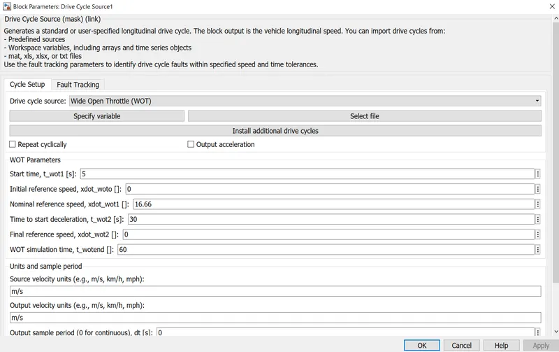
As it is clear from the parameters that the throttle or accelerator of the vehicle is pressed fully between 5-30 seconds time window.
(3) 45 Km/hr for 100 Kms Drive Cycle:
As per the problem statement, a customized drive cycle is made where the vehicle will run with a constant speed of 45 Km/hr and will cover a distance of 100 km approx. The same is implemented by using a signal builder block.
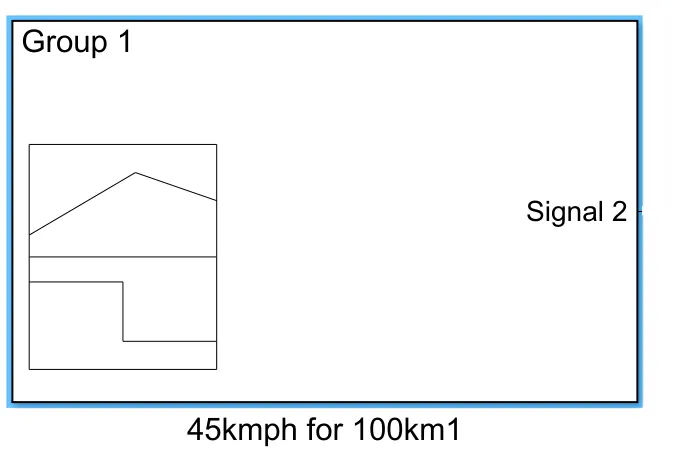
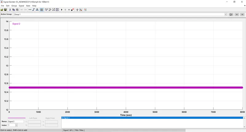
Here the signal builder constant speed is given in approximately 12.5 m/s and run for 8000 Seconds to achieve the 100 km distance covered mark.
(C) Output Obtained From The Simulink Model:
Three drive cycle inputs are given separately, each at a time and their outputs are given separately in different sections.
(C.1) When FTP75 Drive Cycle is the Input:
By giving a '1' value to the multiport switch, we select the FTP75 from the 3 available drive cycles.
(1) Speed Comparison:
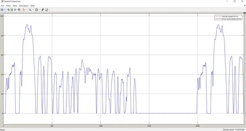
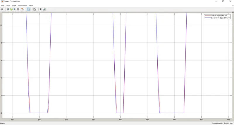
From the above plot, we see the Drive Cycle Speed V.S. Vehicle Speed is compared. It clear from the data that the Electrical Vehicle follows the drive cycle data very well as it coincides with the same for all the time and can not be distinguished without zooming in. After zooming in, the little deviation can be found out mainly at the time of braking when the vehicle needs to decelerate and comes to a halt.
(2) Controller & Motor Temperatures:
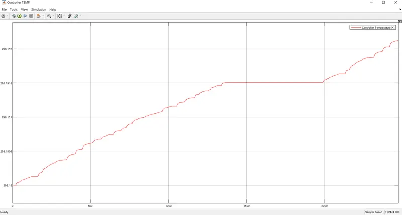
Controller Temperature during operation
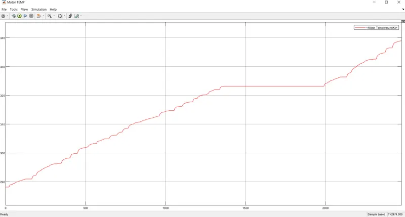
Motor Temperature during operation
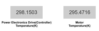
The controller and motor temperature are connected to separate displays to monitor the reading throughout the entire operation and the displays are shown below for the final temperatures at the end of the operation :
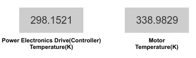 Both in Deg Kelvin
(3) Battery SOC Status:
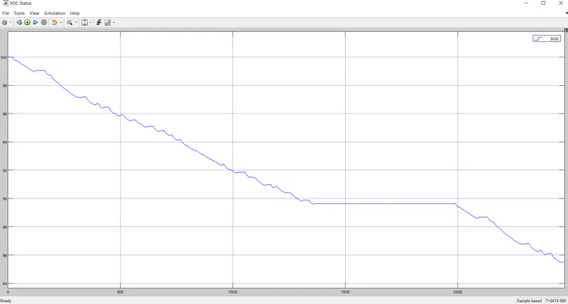
The battery's state of charge or SoC percentage is given in the upper plot where by looking at the discharging and charging one can tell where the vehicle is accelerating or regenerative braking is applied.
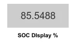
A display is connected to the SoC % output, to monitor it throughout the operation. After the completion of the simulation, the SoC % is found out to be 85.55 % approximately.
(4) Battery Current and Voltage Outputs:
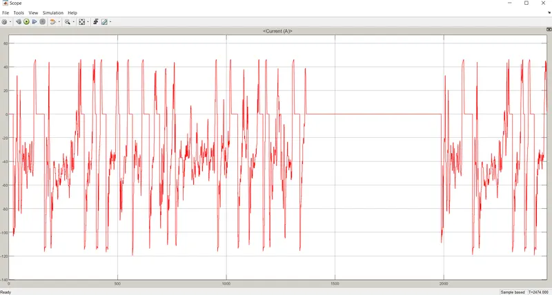
Battery Current
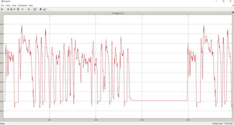
Battery Voltage
Here, Battery current and voltage graphs for the entire process are given. The acceleration of the vehicle denoted the sudden increase in voltage and increase in current in the positive direction; whereas the regenerative braking is indicated by lower voltage changes and the current increase in the negative direction or where the battery gets the charge from the braking action.
(5) Total Distance Covered:
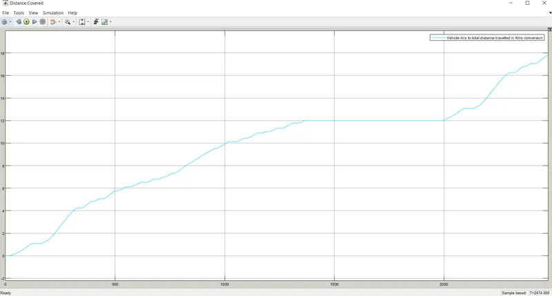
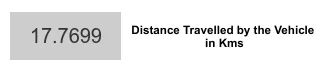
The total distance covered by the vehicle is observed from the graph and for constant monitoring a display is also attached to it, giving the final reading of 17.77 km approximately.
(C.2) When WOT Drive Cycle is the Input:
By giving a '2' value to the multiport switch, we select the WOT from the 3 available drive cycles.
(1) Speed Comparison:
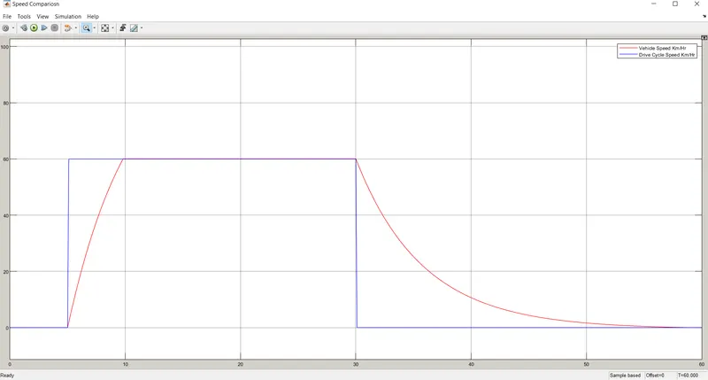
From the above graph, we can see that WOT is given to the input of the driver controller as the drive cycle data. Here, the throttle is fully pressed from 5 seconds to 30 seconds and the corresponding vehicle speed data was tracked. Due to practically the vehicle needs some time to both accelerate to a certain point as well as to decelerating to a point, due to its inertia. Here, in this graph, the vehicle speed is tracking well considering the practicality. It accelerates to the highest point in 10 seconds and then decelerates to rest at 55th second approximately.
(2) Controller & Motor Temperatures:
Controller Temperature
Motor Temperature
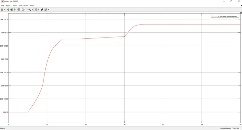
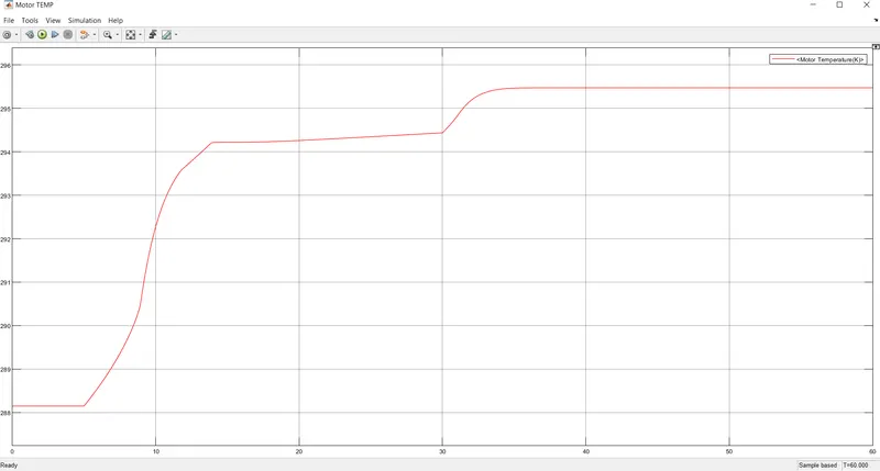
The temperature of both the motor and the controller is raised during the operation and shows the highest reading at the end of the operation. The temperature is increased gradually for the 5 seconds to 10-sec mark and settles to more of a constant during the 10 sec to 30sec mark. And then again is raised slightly due to the braking is applied and ultimately settles down to constant. Both the temperature are connected to separate displays for constant monitoring.
(3) Battery SOC Status:
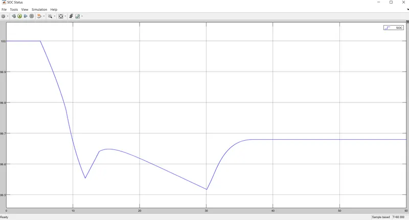
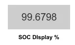
Battery SOC graph is given along with the display to monitor it in real-time. Since it is run for a very lesser amount of time that's why soc percentage only reduces 0.32% approximately.
(4) Battery Current and Voltage Outputs:
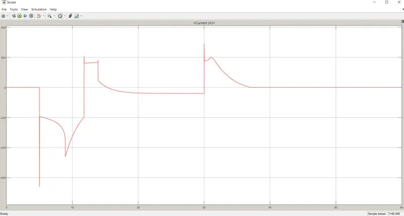
Battery Current
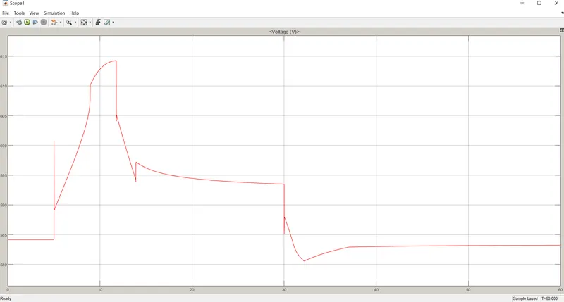
Battery Voltage
In the above graphs, the battery Current and Voltage responses are given for the WOT drive cycle.
(5) Total Distance Covered:
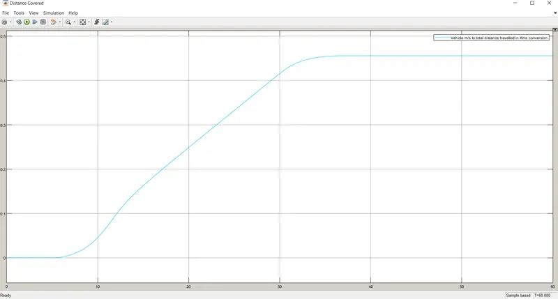
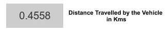
The total distance covered graph and display is given and from the display, one can see that it only traveled for 0.456 km approximately.
(C.3) When Constant 45Km/Hr(for 100 km) Drive Cycle is the Input:
By giving a '3' value to the multiport switch, we select the 45 Km/hr customized drive cycle from the 3 available drive cycles.
(1) Speed Comparison:
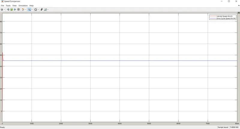
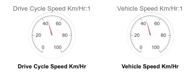
The 45 km/hr speed is maintained by the vehicle during the entire 8000 seconds of operation. From the graph, we can see that the vehicle tracks the drive cycle accurately. Also, to give accuracy two dashboard analog displays were given and you can clearly see that both of them are pointing speed at 45 km/hr. A little overshoot can be seen that is mainly because we are giving instant 45 km/hr speed at both sec at a glance, but for a low-time model it can be used without any problem.
(2) Controller & Motor Temperatures:
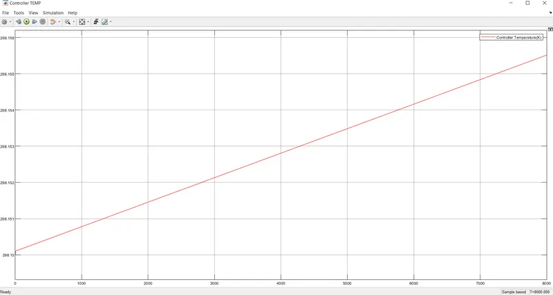
Controller Temperature
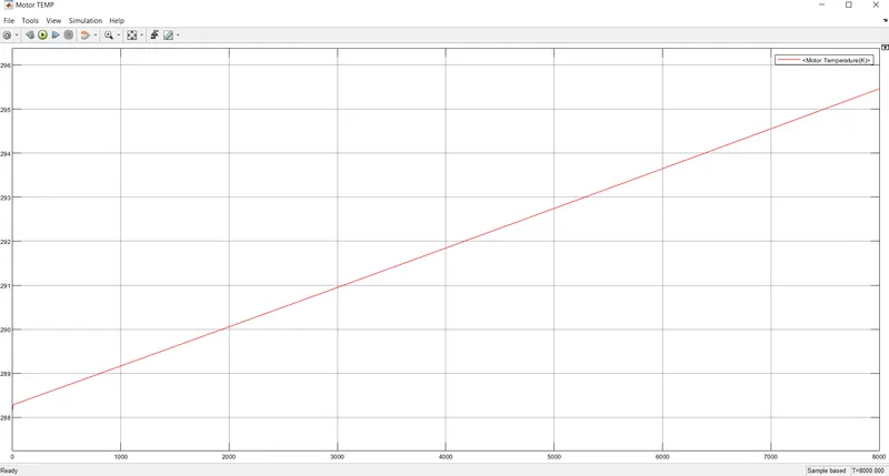
Motor Temperature
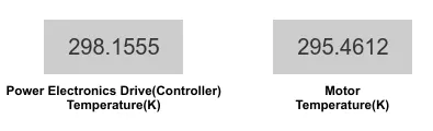
If we look at the graphs, the temperature in both of them is increased at a fixed slope due to its fixed 45 km/hr fixed value. The displays are there to monitor it throughout the process and give the final values as below:
(3) Battery SOC Status:
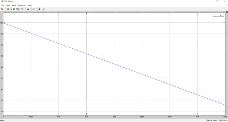
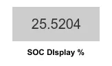
The battery capacity of a small electric 4 wheeler electric vehicle is lesser than a standard one; so after a 100 km journey at 45 km/hr speed drains about 3/4 th of the chargecompletely. It also has to be noted that due to the vehicle's constant speed, there was no regenerating braking was taking place which can further charge the battery during the journey; otherwise, the SOC % maybe end up higher at the end. The SOC percentage is given below with the help of a display block :
(4) Battery Current and Voltage Outputs:
Battery Current
Battery Voltage
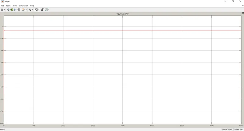
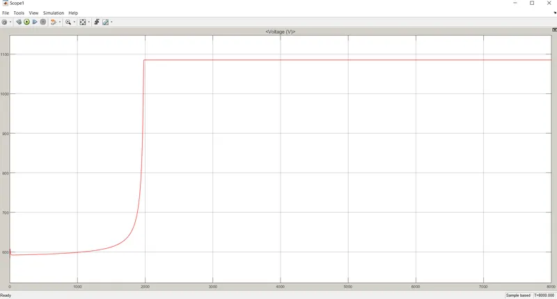
Due to the constant speed, the current and voltages drawn from the battery will also give us constant readings.
It is to be noted that during the initial 0th second, there are both high surges for the voltage and current readings which is not acceptable for a practical scenario but when comes to a low time and simple Simulink model it is acceptable. But it bothers that much one can practically increase the speed to 45 km/hr, taking few seconds to catch up the speed. In this way, there will be no current or voltage surge in this huge amount. This is neglected here because it is not one of the main factors of the given objectives.
(5) Total Distance Covered:
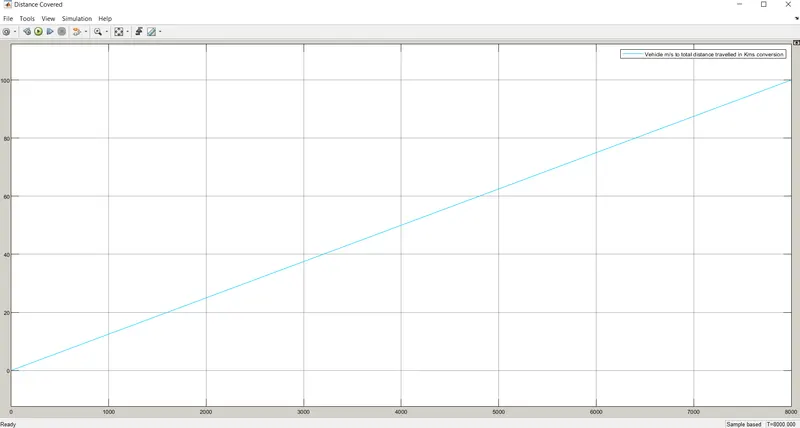
The distance covered can be seen as an increasing straight line with a constant slope. The display block given in below helps us to see the distance covered in real-time. After simulation, it has covered 100 km of distance.

Conclusions: All the necessary theories, description, and parameter details are given for each of the blocks which are used in the Simulink model. All the necessary input-output data are provided for each of FTP75, WOT, and 45 km/hr speed drive cycles with the needed PI controller actions.
Simulink Model: https://drive.google.com/file/d/1L-Kokww9r57Gjdx7NlkA7iFsd8IBRh7u/view?usp=sharing
References:
- https://www.researchgate.net/figure/Parameters-of-the-EV-and-battery_tbl1_270620948https://piaggio-cv.co.in/apeelectrik/?page_id=4147
- https://en.wikipedia.org/wiki/FTP-75#FTP-75
- https://en.wikipedia.org/wiki/Wide_open_throttle#:~:text=Wide%20open%20throttle%20or%20wide,combustion%20engine%20or%20steam%20engine).
- https://en.wikipedia.org/wiki/Proportional_control