INTRODUCTION:
As from the name Hybrid Electric Vehicle, we know that the vehicle is powered using both IC Engine and Electric motor which helps to get great fuel efficiency. By the position of the electric motor that used to power the powertrain we can classified it into different category, so here we are going to the P1 type architecture. The P1 architecture, with the electric motor is connected directly to the crankshaft. This type of architecture helps to act as a starter motor, it also acts as a generator during deceleration, and also helps to give extra power to the engine during vehicle accelerations. It can also provide high torque. Here we are going to monitor the system adopted by the Honda on there first-generation Integrated Motor Assist (IMA) technology. Data is taken from ADVISOR data base developed by NREL, USA. Data provided in the project files. They are using PMSM motor with Power of 10kW and battery capacity of 6Ah, 154V, NiMH Battery.
Load the project2 file to the current folder of the Matlab
Then run the initial file “Project2_InitFile.m” in Matlab script
and then select 1 for the UDDS cycle and 2 for HWFET
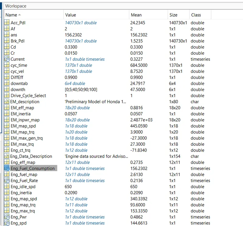
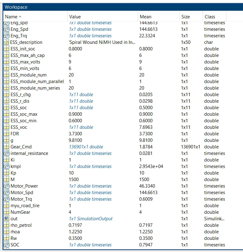
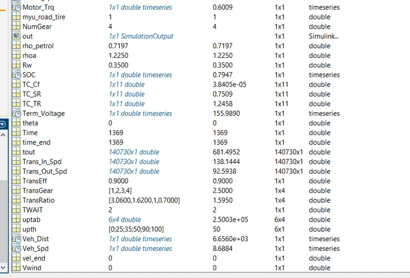
then run the program and bring all data to the workspace.
FOR HWFET
MatLab programme given below for HWFET.
%%%%%%%%%%%%%%%%%%%%%%%%%%%%%%%%%%%%%%%%%%%%%%%%%%%%%%%%%%%%%%%%%%%%%
%% Skill-Lync -> Hybrid Drives Development
% Project 1 - Conventional Vehicle Model
% By - Ullekh Gambhira
% Description:
%% Initialization File
% Initialization file for loading the variables for the Conventional vehicle simulation model
%% Vehicle Parameters
M = 1500; % Vehicle weight [kg]
Cr = 0.015; % Rolling resistance coefficient
Rw = 0.35; % Rolling radius [m]
Cd = 0.33; % Drag coefficient
Af = 2; % Frontal area [m2]
rhoa = 1.225; % Air density [kg/m3]
Vwind = 0; % Wind velocity [kmph]
g = 9.81; % Gravitational acceleration [m/s2]
theta = 0; % Slope [deg]
myu_road_tire = 1; % Coefficient of friction between tire - road interface
%% Data Analysis
Eng_Pwr = Eng_Spd*pi/30*Eng_Trq/1000; % Engine brake power [kW]
rho_petrol = 0.7197; % Density of petrol [kg/L]
kmpl = Veh_Dist(end)/(Eng_Fuel_Consumption(end)/1000/rho_petrol); % Fuel economy [kmpl]
%% Powertrain Parameters
FDR = 3.73; % Final Drive Ratio / Diff Ratio
DiffEff = 0.99; % Differential efficiency (assumed independent of operating conditions)
NumGear = 4; % Number of gears in transmission
TransGear = [1:NumGear]; % Transmission Gears
TransRatio = [3.06, 1.62, 1, 0.7]; % Corresponding Transmission ratios
TransEff = 0.90; % Transmission efficiency (assumed independent of operating conditions)
TC_SR = [0, .5, .6, .7, .8, .87, .92, .94, .96, .97, 1]; % Torque Converter Speed Ratio (Matlab default) -> TurbSpd/PumpSpd
TC_TR = [2.232, 1.5462, 1.4058, 1.2746, 1.1528, 1.0732, 1.0192, 1, 1, 1, 1]; % Torque Converter Torque Ratio (Matlab default) -> TurbTrq/PumpTrq
TC_Cf = 1e-4 * [.72558, .66322, .63463, .59042, .51331, .4144, .29287, .22444, .12186, .04386, 0]; % Torque Converter Capacity Factor (Matlab default) -> PumpTrq/PumpSpd^2 [Nm/rpm^2]
load Vehicle_Data/Engine_data_1_9L_Saturn_95kW
load Vehicle_Data/Trans_Shift_map
load Vehicle_Data/EM_Honda_Insight_10kW
load Vehicle_Data/ESS_NiMH6
ESS_init_soc = 0.8;
ESS_soc_max = 0.9;
ESS_soc_min = 0.6;
%% Driver Parameters
Kp = 10; % P gain for driver PI model
Ki = 1; % I gain for driver PI model
Drive_Cycle_Select = 2; % Drive cycle selection
% Drive cycle values in m/s
if Drive_Cycle_Select == 1
load DriveCycles/UDDS;
elseif Drive_Cycle_Select == 2
load DriveCycles/HWFET;
elseif Drive_Cycle_Select == 3
load DriveCycles/FTP;
elseif Drive_Cycle_Select == 4
load DriveCycles/US06;
elseif Drive_Cycle_Select == 5
load DriveCycles/NEDC;
elseif Drive_Cycle_Select == 6
load DriveCycles/WLTP;
end
time_end = cyc_time(end);
vel_end = cyc_vel(end);
FOR UDDS
MatLab programme given below for UDDS.
%%%%%%%%%%%%%%%%%%%%%%%%%%%%%%%%%%%%%%%%%%%%%%%%%%%%%%%%%%%%%%%%%%%%%
%% Skill-Lync -> Hybrid Drives Development
% Project 1 - Conventional Vehicle Model
% By - Ullekh Gambhira
% Description:
%% Initialization File
% Initialization file for loading the variables for the Conventional vehicle simulation model
%% Vehicle Parameters
M = 1500; % Vehicle weight [kg]
Cr = 0.015; % Rolling resistance coefficient
Rw = 0.35; % Rolling radius [m]
Cd = 0.33; % Drag coefficient
Af = 2; % Frontal area [m2]
rhoa = 1.225; % Air density [kg/m3]
Vwind = 0; % Wind velocity [kmph]
g = 9.81; % Gravitational acceleration [m/s2]
theta = 0; % Slope [deg]
myu_road_tire = 1; % Coefficient of friction between tire - road interface
%% Data Analysis
Eng_Pwr = Eng_Spd*pi/30*Eng_Trq/1000; % Engine brake power [kW]
rho_petrol = 0.7197; % Density of petrol [kg/L]
kmpl = Veh_Dist(end)/(Eng_Fuel_Consumption(end)/1000/rho_petrol); % Fuel economy [kmpl]
%% Powertrain Parameters
FDR = 3.73; % Final Drive Ratio / Diff Ratio
DiffEff = 0.99; % Differential efficiency (assumed independent of operating conditions)
NumGear = 4; % Number of gears in transmission
TransGear = [1:NumGear]; % Transmission Gears
TransRatio = [3.06, 1.62, 1, 0.7]; % Corresponding Transmission ratios
TransEff = 0.90; % Transmission efficiency (assumed independent of operating conditions)
TC_SR = [0, .5, .6, .7, .8, .87, .92, .94, .96, .97, 1]; % Torque Converter Speed Ratio (Matlab default) -> TurbSpd/PumpSpd
TC_TR = [2.232, 1.5462, 1.4058, 1.2746, 1.1528, 1.0732, 1.0192, 1, 1, 1, 1]; % Torque Converter Torque Ratio (Matlab default) -> TurbTrq/PumpTrq
TC_Cf = 1e-4 * [.72558, .66322, .63463, .59042, .51331, .4144, .29287, .22444, .12186, .04386, 0]; % Torque Converter Capacity Factor (Matlab default) -> PumpTrq/PumpSpd^2 [Nm/rpm^2]
load Vehicle_Data/Engine_data_1_9L_Saturn_95kW
load Vehicle_Data/Trans_Shift_map
load Vehicle_Data/EM_Honda_Insight_10kW
load Vehicle_Data/ESS_NiMH6
ESS_init_soc = 0.8;
ESS_soc_max = 0.9;
ESS_soc_min = 0.6;
%% Driver Parameters
Kp = 10; % P gain for driver PI model
Ki = 1; % I gain for driver PI model
Drive_Cycle_Select = 1; % Drive cycle selection
% Drive cycle values in m/s
if Drive_Cycle_Select == 1
load DriveCycles/UDDS;
elseif Drive_Cycle_Select == 2
load DriveCycles/HWFET;
elseif Drive_Cycle_Select == 3
load DriveCycles/FTP;
elseif Drive_Cycle_Select == 4
load DriveCycles/US06;
elseif Drive_Cycle_Select == 5
load DriveCycles/NEDC;
elseif Drive_Cycle_Select == 6
load DriveCycles/WLTP;
end
time_end = cyc_time(end);
vel_end = cyc_vel(end);
SIMULINK MODEL:
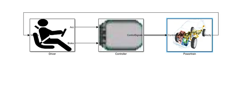
Driver, Controller, Powertrain are three blocks and it’s layout shown above.
Driver:
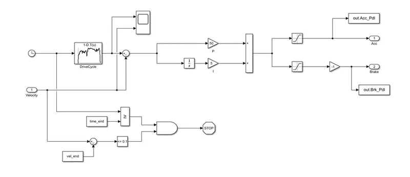
For Driver Block Velocity is input and output is Accelerator (Acc) and Brake. It will control the vehicle velocity by changing the Acc and Brake. Drive data used for Acc and Brake.
Controller Block:
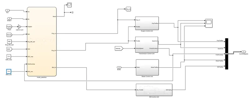
Control block is used to control the Vehicle while driving. Control units are used to control Engine, Transmission, Brake and E-Motor Separately. Working of these units are explained below. Acc and Brake are coming from Driver as Input.
Mode selection:
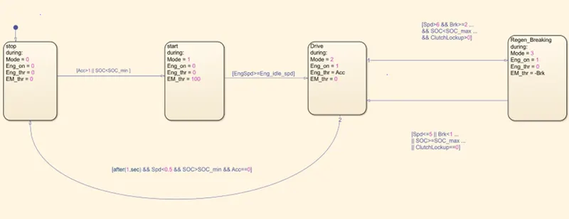
In this chart, different modes like start, stop, driving and Regenerative breaking are given. these modes are changes as per the conditions given in the chart respectively. Mode selection chart given below. Acc and Brake are coming from Driver as Input. Engine Speed, Velocity, SOC min, SOC max, SOC and Engine Idle Speed are given to Mode Selection chart as Input. Engine on, Engine throttle, E-Motor and Mode are outputs.
Engine Control Unit (E.C.U) :
Engine on, Engine Throttle mode is taken as input and E.C.U will control.
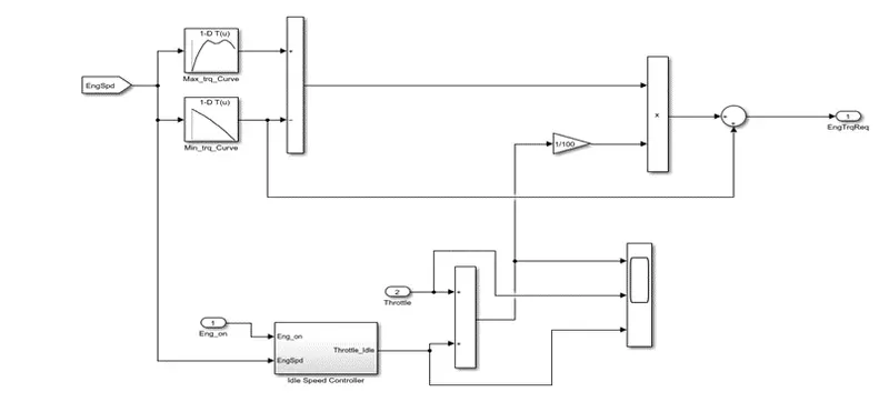
Engine Speed is the input. Eng_map_spd/Eng_max_trq are taken in 1D-Look up table as Max torque curve and Eng_map_spd/Eng_ct_trq are taken in another 1D-Look up table as Min torque curve.
In E.C.U, idle speed controller will be taken if the Engine is on.
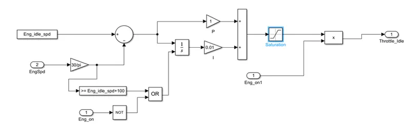
Transmission Control Unit (T.S.U):
For the transmission throttle is open and speed will taken as input. To maintain it steady shift logic is used.
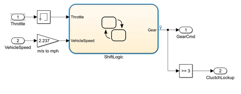
Shift Logic:
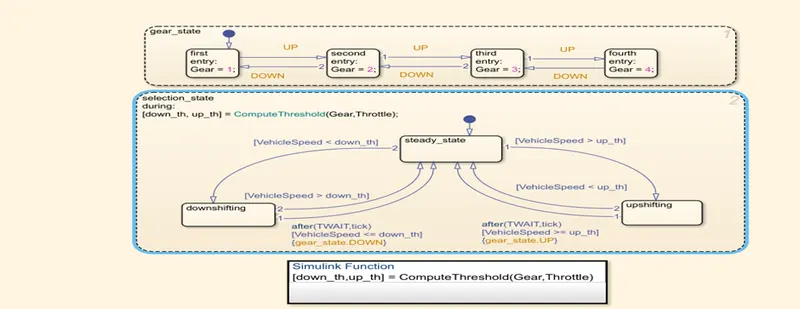
Gear State is controlled by Up shifting and down shifting as given above chart.
Brake Control Unit (B.C.U):
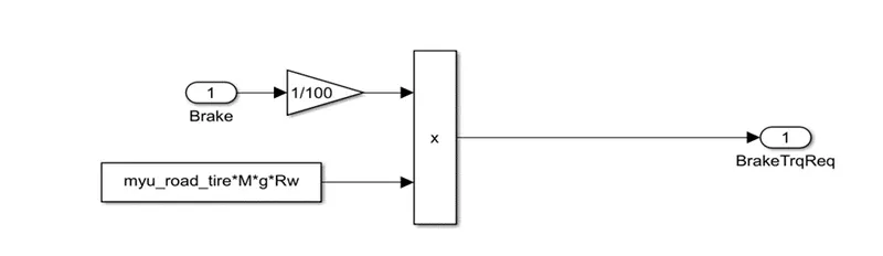
This control unit is used to control the required brake torque. Brake from the Driver is Input.
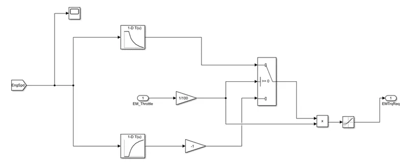
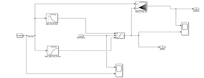
Electric Motor Control Unit (E.M.C.U):
This control unit is used to control the Electric Motor torque required. EM_map_spd is taken as input for the 1-D look up table and outputs are EM_max_trq/EM_max_gen_trq will be selected using switch block. EM Torque required is the output of this control unit.
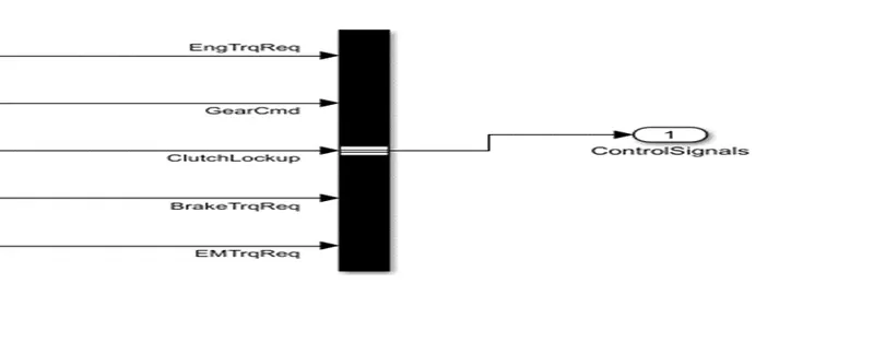
Bus Creator:
The signals from all units are attached to a Bus creator as output of the control unit as shown above.
Powertrain:
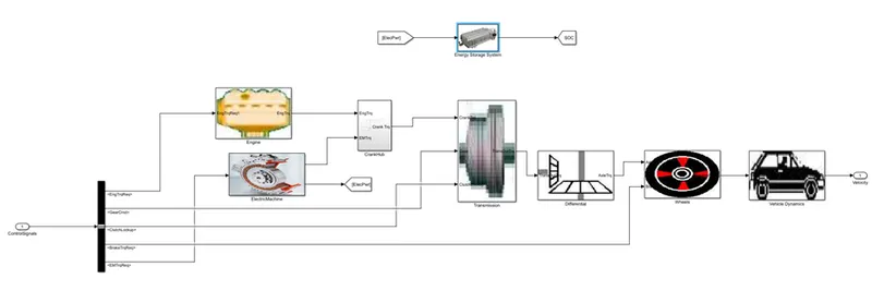
Powertrain will take the input signals from controller block.
Powertrain block consists of following blocks:
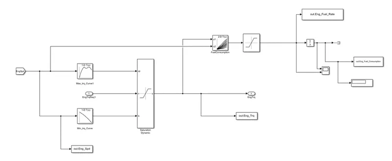
Engine block:
Map based modelling is enabling in this model block, using 1D lookup table the max torque and min torque plotted and then saturated then give a out as fuel consumption and the engine torque.
Electric Motor Block:
Crank Hub:
Transmission:
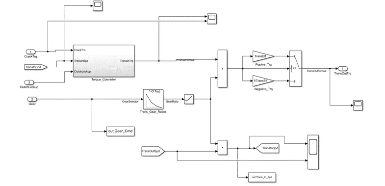
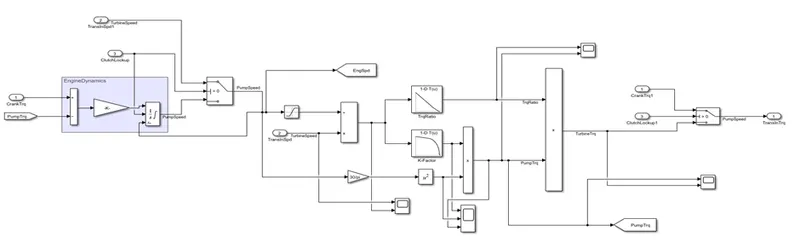
Transmission consists of torque converter.
Torque converter:
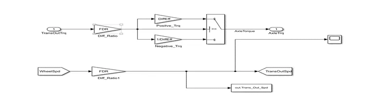
Differential:
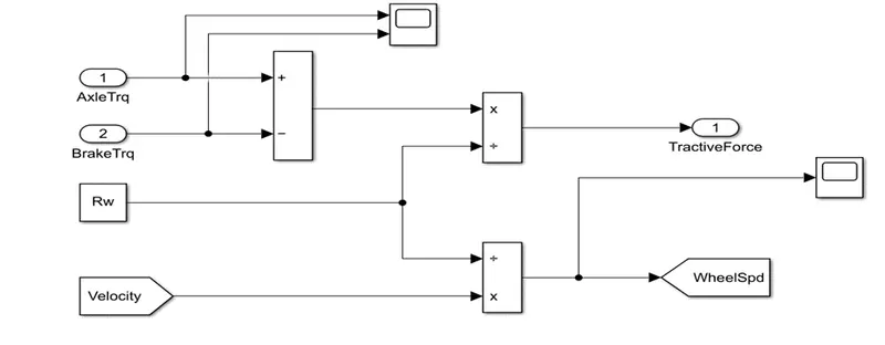
Wheels:
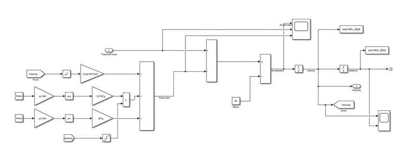
Vehicle Dynamics:
ESS:
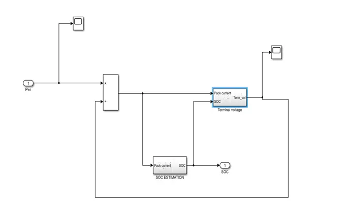
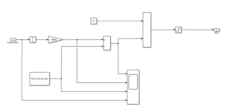
SOC estimation:
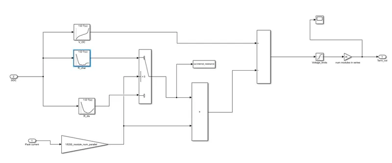
Terminal Voltage:
POST PROCESSING:
POST PROCESSING:
% (b). Plot the time trace for engine, transmission input, transmission output and wheel speed on one plot.
%Time = time_end(end);
Time = out.tout;
figure(1);
hold on
grid on
subplot(4,1,1);
plot(Eng_spd,'LineWidth',2,'Color','black');
ylabel('EngineSpeed');
legend('EngineSpeed');
hold on
grid on
subplot(4,1,2);
plot(Trans_In_Spd, 'linewidth', 1, 'Color', 'black');
ylabel('TransmissionInputSpeed [rpm]')
legend('TransmissionInputSpeed');
hold on
grid on
subplot(4,1,3);
plot(Trans_Out_Spd, 'linewidth', 1, 'Color', 'black');
ylabel('TransmissionOutputSpeed [rpm]')
legend('TransmissionOutputSpeed');
hold on
grid on
subplot(4,1,4);
plot(WheelSpd,'LineWidth',2,'Color','red');
ylabel('WheelSpeed');
legend('WheelSpeed')
%% c. Plot engine torque, engine power, fuel rate and fuel consumption using subplots.
figure(2);
hold on
grid on
subplot(4,1,1);
plot(Eng_Trq,'LineWidth',2,'Color','black');
ylabel('EngineTorque');
legend('EngineTorque');
hold on
grid on
subplot(4,1,2);
plot(Eng_Fuel_Rate, 'linewidth', 1, 'Color', 'black');
ylabel('EngineFuelRate')
legend('EngineFuelRate');
hold on
grid on
subplot(4,1,3);
plot(Eng_Fuel_Consumption, 'linewidth', 1, 'Color', 'black');
ylabel('EngineFuelConsumption')
legend('EngineFuelConsumption');
hold on
grid on
subplot(4,1,4);
plot(Eng_Pwr,'LineWidth',2,'Color','green');
ylabel('EnginePower');
legend('EnginePower')
%% d. Plot accelerator and brake pedal, gear command, vehicle desired and actual speed, vehicle distance using subplots.
figure(3);
title('Plots for accelerator and brake pedal, gear command, vehicle desired and actual speed, vehicle distance ')
hold on
grid on
subplot(4,1,1);
plot(Acc_Pdl,'LineWidth',1,'Color','black');
plot(Brk_Pdl,'LineWidth',1,'Color','red');
ylabel('Pedal');
legend('Accel','Pedal');
hold on
grid on
subplot(4,1,2);
plot(Gear_Cmd,'LineWidth',1,'Color','black');
ylabel('Gear Command');
legend('Gear Command');
hold on
grid on
subplot(4,1,3);
plot(Veh_Spd,'LineWidth',1,'Color','black');
ylabel('Vehicle Speed');
legend('Vehicle Speed');
hold on
grid on
subplot(4,1,4);
plot(Veh_Dist,'LineWidth',1,'Color','red');
ylabel('Vehicle Distance');
legend('Vehicle Distance');
%% e. Plot the engine operating points on the engine fuel map.
figure(4);
hold on
grid on
title('name','Engine Operating points');
p1 = plot(Eng_map_spd*30/pi, Eng_max_trq);
%p2 = plot( [Eng_map_spd(end)*30/pi Eng_max_spd(end)] , [0 Eng_max_trq(end)]);
p2=line([Eng_map_spd(end)*30/pi Eng_map_spd(end)*30/pi],[0 Eng_max_trq(end)]);
p3 = line([Eng_map_spd(1)*30/pi Eng_map_spd(1)*30/pi] , [0 Eng_max_trq(1)]);
[c,h] = contour(Eng_map_spd'*30/pi , Eng_map_trq, Eng_fuel_map');
clabel(c,h);
xlabel('Engine Speed [rpm]');
ylabel('Engine Torque [Nm]');
title('Engine Fuel Consumption Map [g/s]');
p4 = plot(Eng_Spd,'.','color','k');
p4 = plot(Eng_Trq,'.','color','g');
legend([p1 p4],{'Max Curve','Operating Points'});
axis([Eng_map_spd(1)*30/pi Eng_map_spd(end)*30/pi 0 Eng_map_trq(end)]);
%% f. Plot motor speed, torque, motor input power using subplots.
figure(5);
hold on
grid on
subplot(3,1,1);
plot(Motor_Spd,'LineWidth',1,'Color','black');
ylabel('Motor Speed');
legend('Motor Speed');
hold on
grid on
subplot(3,1,2);
plot(Motor_Power,'LineWidth',1,'Color','red');
ylabel('Motor Power');
legend('Motor Power');
hold on
grid on
subplot(3,1,3);
plot(Motor_Trq,'LineWidth',1,'Color','green');
ylabel('Motor Torque');
legend('Motor Torque');
title('Plots for motor speed, torque, motor power');
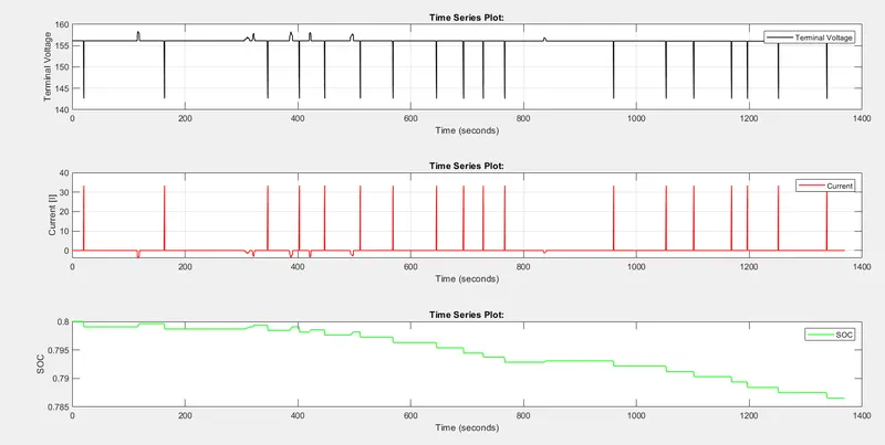
%% g. Plot pack voltage, current and SoC using subplots.
figure(6);
title('Plots for pack voltage, current and SOC ');
hold on
grid on
subplot(3,1,1);
plot(Term_Voltage,'LineWidth',1,'Color','black');
ylabel('Terminal Voltage');
legend('Terminal Voltage');
hold on
grid on
subplot(3,1,2);
plot(Current,'LineWidth',1,'Color','red');
ylabel('Current [I]');
legend('Current');
hold on
grid on
subplot(3,1,3);
plot(SOC,'LineWidth',1,'Color','green');
ylabel('SOC');
legend('SOC');
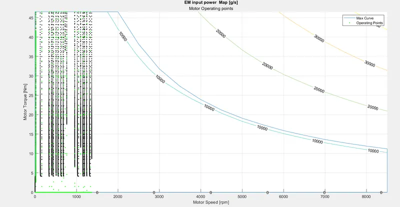
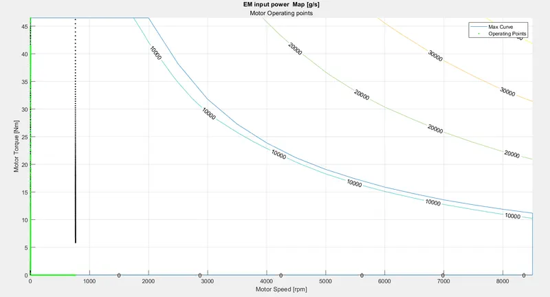
%% h. Plot the motor operating points on the motor input power map, with the motor max motoring and generating torque curves.
figure(7);
hold on
grid on
title('name','Motor Operating points');
p1 = plot(EM_map_spd*30/pi, EM_max_trq);
p2=line([EM_map_spd(end)*30/pi EM_map_spd(end)*30/pi],[0 EM_max_trq(end)]);
p3 = line([EM_map_spd(1)*30/pi EM_map_spd(1)*30/pi] , [0 EM_max_trq(1)]);
[c,h] = contour(EM_map_spd'*30/pi , EM_map_trq, EM_inpwr_map');
clabel(c,h);
xlabel('Motor Speed [rpm]');
ylabel('Motor Torque [Nm]');
title('EM input power Map [g/s]');
p4 = plot(Motor_Spd,'.','color','k');
p4 = plot(Motor_Trq,'.','color','g');
legend([p1 p4],{'Max Curve','Operating Points'});
axis([EM_map_spd(1)*30/pi EM_map_spd(end)*30/pi 0 EM_map_trq(end)]);
%%
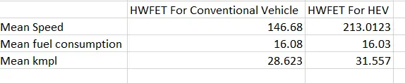
a. Tabulate the fuel economy numbers (kmpl) for UDDS and HWFET cycle. Compare these numbers with the baseline numbers for conventional vehicle model from Project 1.
The fuel economy numbers (kmpl) for HWFET HEV.
HWFET For HEV and Conventional Vehicle:
UDDS For HEV and Conventional Vehicle:

From above observations HEV is giving more Average Speed Compared to Conventional Vehicle in HWFET. But in fuel consumption is almost same is for both vehicles and KMPL is high in HEV's Compared to conventional vehicle. mean speed is more because we are using electric motor in HEV. For UDDS, Mean speed is same for both. but fuel consumption is 10% more efficient than convention vehicle. KMPL is also high in HEV.
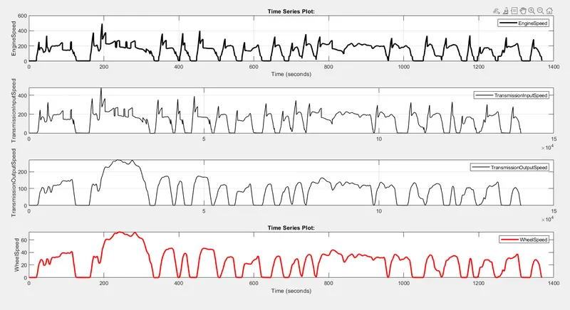
b. Plot the time trace for engine, transmission input, transmission output and wheel speed on one plot.
UDDS:
HWFET:
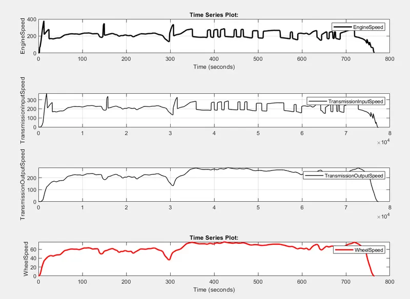
From above Drive Cycles, Engine speed, transmission input and output speed, wheel speeds are high in High ways (HWFET) comparing to Urban areas(UDDS).it is because in urban areas traffics are high and the vehicle need to be stop. Because of it speeds in UDDS cycle becomes zero. HEV’s in High ways will give High speed.
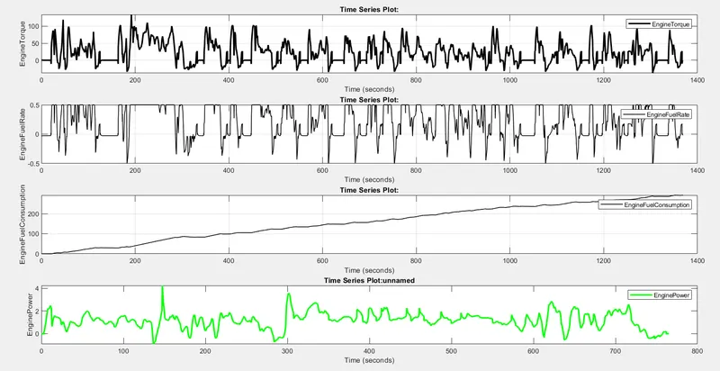
c. Plot engine torque, engine power, fuel rate and fuel consumption using subplots.
UDDS:
HWFET:
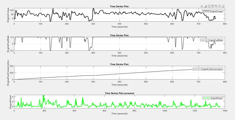
From both HWFET and UDDS Drive cycles, Engine torque in High ways is high comparing to the Urban areas. In Urban areas Engine Torque lines are moving up and down because of traffic in these areas. So, the fuel consumption rate is constant in HWFET because of high torques. Engine Power in urban areas high(due to traffic some power may loss) and in high ways it is low.
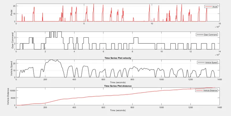
d. Plot accelerator and brake pedal, gear command, vehicle desired and actual speed, vehicle distance using subplots.
UDDS:
HWFET:
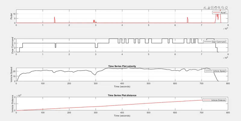
From above both cycles, HEV’s in High ways are getting more speed on increasing the gear and by accelerating. But in UDDS(urban areas) even if we accelerated, the vehicle speed facing some up and downs.
e. Plot the engine operating points on the engine fuel map.
UDDS:
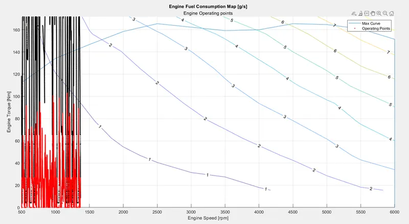
HWFET:
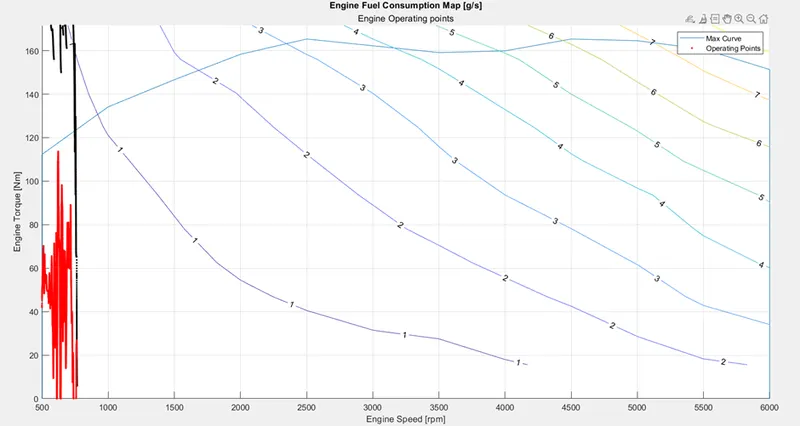
In both drive cycles, for less fuel consumption and the engine speed increasing.
f. Plot motor speed, torque, motor input power using subplots.
UDDS:
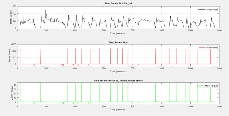
HWFET:
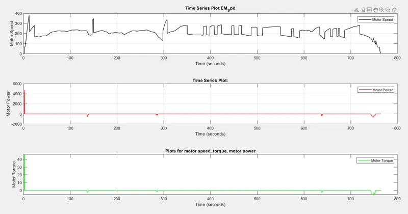
we can see that the power and torque are very high in HWFET at initial condition and they are almost zero after some times but in USSD its has continuos flectuation due to the frequent breaking in ussd cycle.
g. Plot pack voltage, current and SoC using subplots.
UDDS:
HWFET:
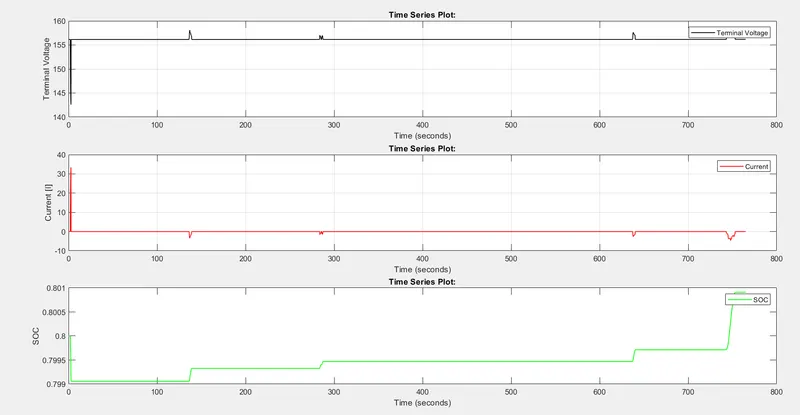
The pack current and terminal voltage will have more flectuation when compare to the HWFET cycle with USSD. it is because of the radip stop and start in city ride where the motor need to work more.
SOC decreases in USSD with time and increases with HWFET.
h. Plot the motor operating points on the motor input power map, with the motor max motoring and generating torque curves.
USSD:
HWFET:
by using the Drive cycles, we find out various charecteristics of HEV's in high ways and urban areas.
following are the questions and answers are given above.
a. Tabulate the fuel economy numbers (kmpl) for UDDS and HWFET cycle. Compare these numbers with the baseline numbers for conventional vehicle model from Project 1.
b. Plot the time trace for engine, transmission input, transmission output and wheel speed on one plot.
c. Plot engine torque, engine power, fuel rate and fuel consumption using subplots.
d. Plot accelerator and brake pedal, gear command, vehicle desired and actual speed, vehicle distance using subplots.
e. Plot the engine operating points on the engine fuel map.
f. Plot motor speed, torque, motor input power using subplots.
g. Plot pack voltage, current and SoC using subplots.
h. Plot the motor operating points on the motor input power map, with the motor max motoring and generating torque curves.
Thank you,
Skill Lync