Project 2
Hypothesis:
P1 Mild Hybrid Electric Vehicle:
The Pl design, with the electric machine associated straightforwardly to the driving rod, is the arrangement taken on by Honda on their original Integrated Motor Assist (IMA) innovation. The electric engine capabilities as a generator, during vehicle deceleration, as a motor starter, and as an engine (to help the motor) during vehicle speed increases. One of the greatest benefits of this arrangement is that the electric engine can give higher force than the BISG, since there is no belt impediment (because of slip). In any case, since there is no speed/force proportion between the electric machine and driving rod, the force necessities on the electric engine can very request.
Two instances of PI MHEV models are:
Honda Insight Hybrid 2009 (with Integrated Motor Assist innovation)
Mercedes Benz S400 Bluehybrid 2010
For instance, the fundamental qualities of the PI MHEV.
1] Electric Machine Performance:
Greatest force up to 34 Nm.
Most extreme power: 10KW
Effectiveness: Up to 94 Percent
2] Hybrid Modes:
Inactive endlessly stop
Moving pause and begin
Motor burden shift
Force help
Force support
Energy recovery
Brake age
3] Advantages:
Higher effectiveness
The 12V starter can be eliminated
4] Disadvantages:
Yield force restricted by the size of the electric machine
Energy recovery impacted by motor rubbing misfortunes
High effect on existing vehicle design
Higher generally cost of the electrical parts
Air cooling unrealistic for electric machine
5] Overall attributes:
Force Boosting limit: High
Electrical energy recovery: Medium
Driveability enhancements: Medium
Electrical Creep/drive: Possible
In this model We use Forward Model:
It is otherwise called dynamic reproduction. Dynamic models are utilized for nitty gritty reproductions. In this model power/force/power is the information and the vehicle state variable speed and speed increase are yields. The models and reproductions are more reasonable because of actual setback thus proper for control advancement. There is an input circle to meet the ideal vehicle state. It is basically used to reenact a vehicle on a driving cycle to break down the powerful way of behaving of the framework helps essentially in charge improvement.
1) Load the Project2 folder as the Current Folder in Matlab.
%%%%%%%%%%%%%%%%%%%%%%%%%%%%%%%%%%%%%%%%%%%%%%%%%%%%%%%%%%%%%%%%%%%%%

Skill-Lync -> Hybrid Drives Development
Project 1 - Conventional Vehicle Model By - Ullekh Gambhira
% Description:

Initialization File
Initialization file for loading the variables for the Conventional vehicle simulation model
Vehicle Parameters
M = 1500;       % Vehicle weight [kg]
Cr = 0.015;     % Rolling resistance coefficient
Rw = 0.35;      % Rolling radius [m]
Cd = 0.33;      % Drag coefficient
Af = 2;         % Frontal area [m2]
rhoa = 1.225;   % Air density [kg/m3]
Vwind = 0;      % Wind velocity [kmph]
g = 9.81;       % Gravitational acceleration [m/s2]
theta = 0;      % Slope [deg]
myu_road_tire = 1; % Coefficient of friction between tire - road interface

Powertrain Parameters
FDR = 3.73;                         % Final Drive Ratio / Diff Ratio
DiffEff = 0.99;                     % Differential efficiency (assumed independent of operating conditions)

NumGear = 4;                        % Number of gears in transmission
TransGear = [1:NumGear];            % Transmission Gears
TransRatio = [3.06, 1.62, 1, 0.7];  % Corresponding Transmission ratios
TransEff = 0.90;                    % Transmission efficiency (assumed independent of operating conditions)

TC_SR = [0, .5, .6, .7, .8, .87, .92, .94, .96, .97, 1];   % Torque Converter Speed Ratio (Matlab default) -> TurbSpd/PumpSpd
TC_TR = [2.232, 1.5462, 1.4058, 1.2746, 1.1528, 1.0732, 1.0192, 1, 1, 1, 1];   % Torque Converter Torque Ratio (Matlab default) -> TurbTrq/PumpTrq
TC_Cf = 1e-4 * [.72558, .66322, .63463, .59042, .51331, .4144, .29287, .22444, .12186, .04386, 0]; % Torque Converter Capacity Factor (Matlab default) -> PumpTrq/PumpSpd^2 [Nm/rpm^2]

load Vehicle_Data/Engine_data_1_9L_Saturn_95kW
load Vehicle_Data/Trans_Shift_map
load Vehicle_Data/EM_Honda_Insight_10kW
load Vehicle_Data/ESS_NiMH6


ESS_init_soc = 0.8;
ESS_soc_max = 0.9;
ESS_soc_min = 0.6;

Driver Parameters
Kp = 10;                    % P gain for driver PI model
Ki = 1;                     % I gain for driver PI model
Drive_Cycle_Select = 2;     % Drive cycle selection

% Drive cycle values in m/s

if Drive_Cycle_Select == 1
    load DriveCycles/UDDS;

elseif Drive_Cycle_Select == 2
    load DriveCycles/HWFET;

elseif Drive_Cycle_Select == 3
    load DriveCycles/FTP;

elseif Drive_Cycle_Select == 4
    load DriveCycles/US06;

elseif Drive_Cycle_Select == 5
    load DriveCycles/NEDC;

elseif Drive_Cycle_Select == 6
    load DriveCycles/WLTP;

end

time_end = cyc_time(end);
vel_end = cyc_vel(end);
Vehicle
Layout
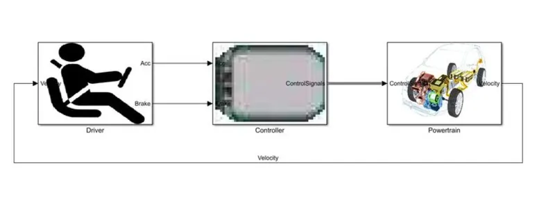
Driver
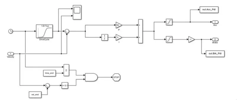
Controller
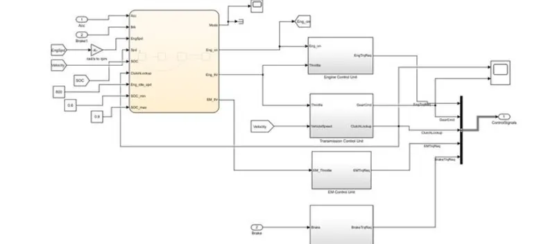
Stateflow for Controller
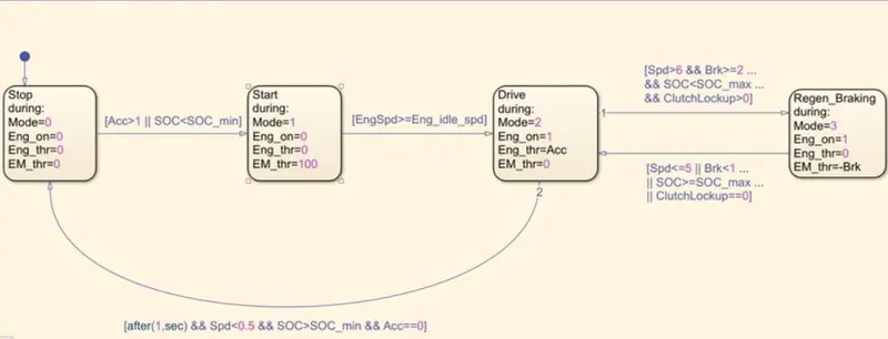
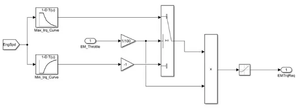
In this we made four circumstances as stop, begin, drive and regenerative slowing down. The underlying block addresses the stop condition. In which the motor is off. The motor and engine choke conditions are zero. Then the subsequent block addresses the beginning condition. In which the mode is 1 the electric engine choke is simply used to give the necessary force and capacity to the vehicle. The motor is off and motor choke condition zero.The state 1 and state 2 are associated utilizing the connections for example it moves from state 1 to state 2 when speed increase is short of what one or SOC is less then the base SOC.State 3 Represents mode 2 ii.e. motor is on and the motor choke is likewise having positive worth from the driver yet the electric engine choke is zero. It changes structure state 2 to state 3 when motor speed is more prominent than or equivalent to motor stand-by speed.
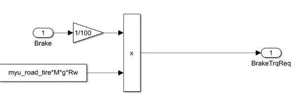
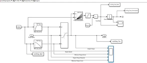
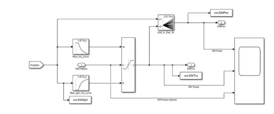
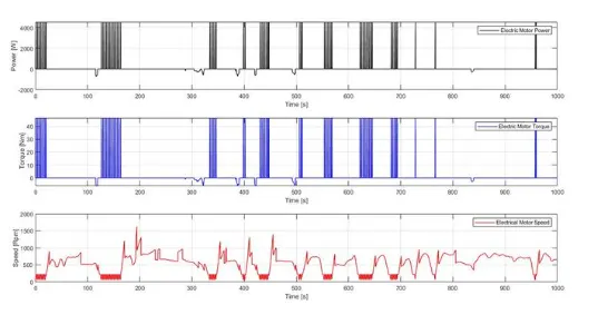
State 4 addresses regenerative slowing down which is model 3 In this express the motor is on however the motor choke is having no contribution from the driver though the electric engine gets the negative power because of braking.The inputs given to the graph are Acceleration, barke, motor speed, vehicle speed, SOC, and grip lockup.The yield we get from the outline is mode, motor condition, motor choke condition, and electric engine choke condition.Modification done in all Unit displaying. they displayed in the following figures.
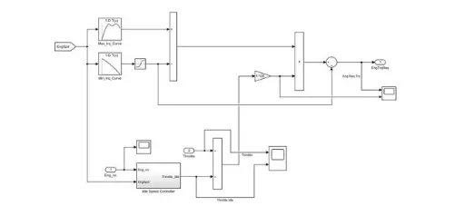
Engine Control Unit
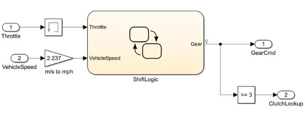
Transmission Control Unit
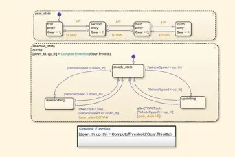
Shiftlogic in this unit
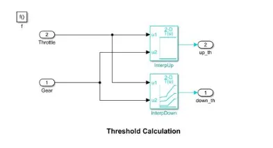
Threshold value in this controller
Electric Motor Control unit
Brake Control unit
Engine
Electric Motor
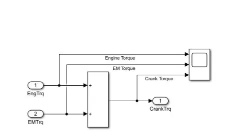
Crankhub
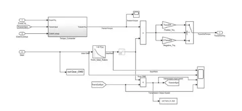
Transmission
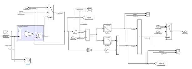
Torque Converter
Differential
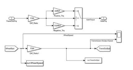
Wheel
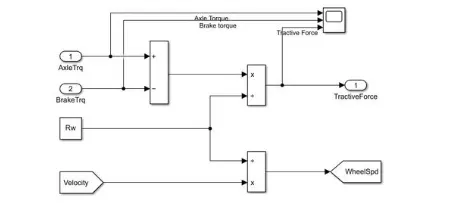
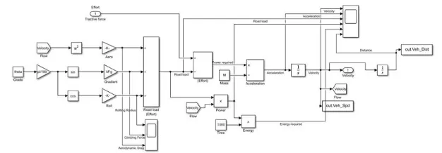
Vehicle Dynamics
Battery Modelling
Storage system
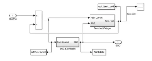
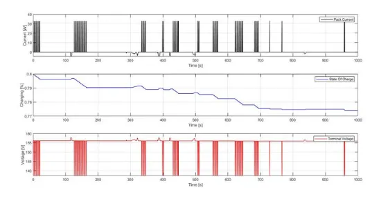
Terminal Voltage
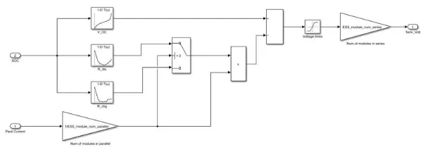
Pack Current
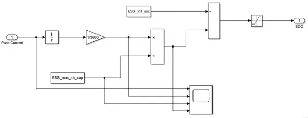
Code for creating Plots
%% Renaming variables
Time=out.tout;
Acc_Pd1=out.Acc_Pd1; % Accelerator pedal [%]
Brk_Pd1=out.Brk_Pdl;% Brake pedal [%]
Gear_Cmd=out.Gear_CMD;% Transmission gear
Trans_In_Spd=out.Trans_In_Spd*30/pi; % Transmission input speed [rpm]
Trans_Out_Spd=out.TransOutSpd*30/pi;% Transmission output speed [rpm]
Eng_Trq=out.Eng_Trq;% Engine brake torque [Nm]
Eng_Spd=out.Eng_Spd*30/pi; % Engine speed [rpm]
Eng_Fuel_Consump=out.Eng_Fuel_Consumption; % Engine fuel consumption [g]
Veh_Dist=out.Veh_Dist/1000;% Distance traveled by vehicle [km]
Veh_Spd=out.Veh_Spd*18/5;% Vehicle speed [kmph]
Wheel_Speed=out.WheelSpeed; % Wheel speed [kmph] Eng_Fuel_Rate = out. Eng_Fuel_Rate % Engine fuel rate [%]
EM_Speed=out.EMSpd*18/5;% Electric Motor Speed
EM_Power=out.EMPwr;% Electric Motor Power
EM_Torque=out.EMTrq;% Electric Motor Torque
Term_Volt=out.term_volt;%Terminal Voltage of battery
Soc=out.SOC;% State Of Charge
Pack_Current=out.Pack_Current;%Pack current of battery


%% Data Analysis
Eng_Pwr=Eng_Spd*pi/30*Eng_Trq/1000; % Engine brake power [kW]
rho_petrol = 0.7197;% Density of petrol [kg/L]
kmpl=Veh_Dist(end)/(Eng_Fuel_Consump(end)/1000/rho_petrol);% Fuel economy [kmpl]

%% Plotting vehicle characteristics time trace to Engine speed, Engine Torque, Engine Power,
% And Engine fuel rate, Engine fuel consumption
% Data conversion from Double Timeseries
Eng_spd = Eng_Spd.Data(:,1); % engine speed
Eng_trq = Eng_Trq.Data(:,1); % engine torque
Eng_pwr = Eng_Pwr.Data(:,1); % engine power Eng_fuel rate = Eng_Fuel_Rate.Data(:,1); % engine fuel rate
Eng_fuel_consumption=Eng_Fuel_Consump.Data(:,1); %engine fuel consumption
EM_speed=EM_Speed.Data(:,1); % motor speed
EM_power=EM_Power.Data(:,1); % Motor Power
EM_torque=EM_Torque.Data(:,1); % Motor Torque =
Pack_current=Pack_Current.Data(:,1); %pack current of battery =
State_of_charge=Soc.Data(:,1); %state of charge =
Term_voltage=Term_Volt.Data(:,1);%terminal Voltage of battery


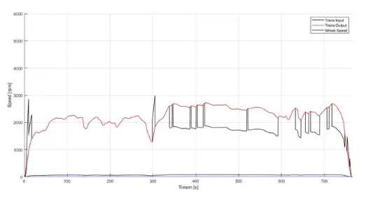
%% Plotting vehicle characteristics time trace transmission IN/OUT and Wheel Speed

figure(1)
hold on
grid on
plot(Time,Trans_In_Spd,'linewidth',1,'Color','black');
plot(Time,Trans_Out_Spd,'linewidth',1,'Color','red');
plot(Time,Wheel_Speed,'linewidth',1,'color','blue')
ylabel('Speed[rpm]')
xlabel('Timem[s]')
xlim([0, Time (end)]);
ylim([0, 6000]);
legend('Trans Input', 'Trans Output', 'Wheel Speed');

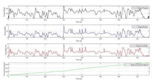
%% Plotting Engine speed, Engine Torque, Engine Power, Engine fuel rate, Engine fuel consumption wrt Time

figure(2)
subplot(4,1,1)
plot(Time,Eng_trq,'linewidth',1,'color','black')
xlim([0, Time (end)]);
xlabel('Time [s]')
ylabel('Torque [Nm]')
legend('Engine Torque')
grid on
subplot (4,1,2)
plot(Time,Eng_pwr,'linewidth',1,'color','blue')
xlim([0, Time (end)]);
xlabel('Time[s]')
ylabel('Power[KW]')
legend('Engine Power')
grid on

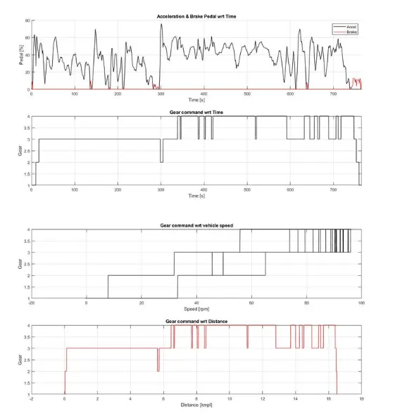
%% Potting Accelerator pedal, Brake pedal and gear command with respect to time
figure(4)
subplot(2,1,1)
hold on
plot(Time, Acc_Pdl,'linewidth',1,'Color','black');
plot (Time, Brk_Pdl,'linewidth',1,'Color','red');
ylabel('Pedal [%]')
xlabel('Time [s]');
xlim([0, Time (end)]);
grid on
legend('Accel','Brake');
title('Acceleration & Brake Pedal wrt Time')
subplot(2,1,2)
plot (Time,Gear_Cmd,'linewidth',1,'Color','black');
xlim([0, Time (end)]);
xlabel('Time[s]');
ylabel('Gear');
grid on
title('Gear command wrt Time')

% Plotting gear command vehicle desired with actual speed
figure(5)
subplot(2,1,1)
plot(Veh_spd,Gear_Cmd,'linewidth',1,'Color','black');
xlabel('Speed[rpm]');
ylabel('Gear');
grid on
title('Gear command wrt vehicle speed')
subplot(2,1,2)
plot (Veh_dist,Gear_Cmd,'linewidth',1,'Color','red');
xlabel('Distance [kmpl]');
ylabel('Gear');
grid on
title('Gear command wrt Distance')

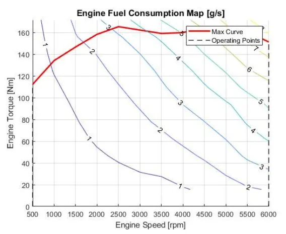
%% Plotting engine operating points on engine fuel map figure('Name', 'Engine Operating Points');
hold on
grid on
title('Engine Operating Points', 'fontsize', 12);
p1=plot (Eng_map_spd*30/pi,Eng_max_trq,'linewidth',2,'color','r');
p2=line([Eng_map_spd (end)*30/pi Eng_map_spd (end)*30/pi], [0 Eng_max_trg (end)]);
set(p2,'linewidth',1,'linestyle','--','color','k');
p3=line([Eng_map_spd (1)*30/pi Eng_map_spd (1)*30/pi], [0 Eng_max_trq(1)]);
set(p3,'linewidth',1, 'linestyle','-','color','k');
[c,h]=contour(Eng_map_spd'*30/pi,Eng_map_trq,Eng_fuel_map');
clabel(c,h);
xlabel('Engine Speed [rpm]');
ylabel('Engine Torque [Nm]');
title('Engine Fuel Consumption Map [g/s]');
legend([p1 p3],['Max Curve','Operating Points'});
axis([Eng_map_spd(1)*30/pi Eng_map_spd(end)*30/pi 0 Eng_map_trq(end)]);

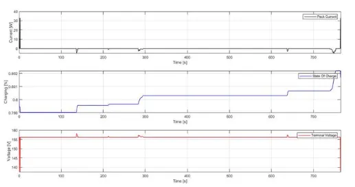
%% State of Charge, Pack Current, And Terminal Voltage with respect to Time
figure(6)
subplot (3,1,1)
plot(Time,Pack_current,'linewidth',1,'color', 'black')
xlim([0,Time(end)]);
xlabel('Time [s]')
ylabel('Current [W]')
legend('Pack Current')
grid on

subplot(3,1,2)
plot(Time,State_of_charge,'linewidth',1,'color','blue')
xlim([0, Time (end)]);
xlabel('Time[s]')
ylabel('Charging [%]')
legend('State Of Charge')
grid on

subplot (3,1,3).
plot (Time,Term_voltage, 'linewidth',1,'color', 'red')
xlim([0,Time (end)]);
xlabel('Time[s]')
ylabel('Voltage[V]')
legend('Terminal Voltage')
grid on

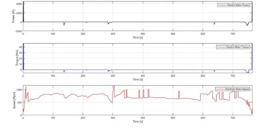
%% Motor Speed, Torque, Motor input power with respect to Time
figure(7)
subplot(3,1,1)
plot(Time,EM_power,'linewidth',1,'color','black')
xlim([0, Time (end)]);
xlabel('Time[s]')
ylabel('Power[W]')
legend('Electric Motor Power ')
grid on

subplot(3,1,2)
plot(Time,EM_torque,'linewidth',1,'color','blue')
xlim([0,time(end)]);
xlabel('Time[s]')
ylabel('Torque[Nm]')
legend('Electric Motor Torque')
grid on

subplot(3,1,3)
plot(Time,EM_speed,'linewidth',1,'color','red')
xlim([0,Time(end)]);
xlabel('Time[s]')
ylabel('Speed[Rpm]')
legend('Electrical Motor Speed')
grid on

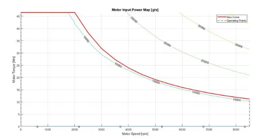
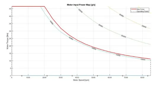
%% Plotting EM Operating Points on motor input power Map figure( 'Name', 'Electric Motor Operating Points');
hold on
grid on
title('Electric Motor Operating Points','fontsize', 12);
pl=plot(EM_map_spd*30/pi,EM_max_trq,'linewidth',2,'color','r');
p2=line([EM_map_spd (end)*30/pi EM_map_spd(end) *30/pi],[0 EM_max_trg (end)]);
set(p2, 'linewidth',1,'linestyle','-','color','k');
p3=line([EM_map_spd (1)*30/pi EM_map_spd (1)*30/pi],[0 EM_max_trq(1)]);
set(p3,'linewidth',1,'linestyle','-','color','k');
[c,h]=contour(EM_map_spd**30/pi,EM_map_trq,EM_inpwr_map');
clabel(c,h);
xlabel('Motor Speed[rpm]');
ylabel('Motor Torque[Nm]');
title('Motor Input Power Map [g/s]');
legend([p1 p3], ['Max Curve', 'Operating Points'});
axis([EM_map_spd(1)*30/pi EM_map_spd (end)*30/pi 0 EM_map_trg(end)]);
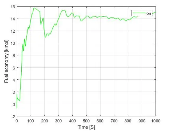
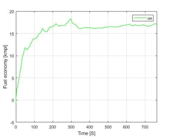
Fuel Economy Numbers for project 2
S.No
Drive cycle
Fuel Economy Number (KMpl)
UDDS=15.0773
HWFET=17.1613
As we see the fuel economy is high in HWFET compared to UDDS. It is because in urban driving the vehicle encounters more traffic and it has to stop for a greater distance and it consumes more fuel at the starting. In HWFET the vehicle encounters no traffic and it moves without use of too much braking so it will have more fuel economy number.
Comparing with fuel economy numbers for project 1
S.No
Drive cycle
UDDS=14.209
HWFET=16.503
As we see the fuel economy numbers for project 2 are a bit higher when compared to project 1 because of implementing the electric motor as it is Pl hybrid it may not have much variation in the fuel economy but as we implement other architectures it will increase by huge amount.
Plots for UDSS
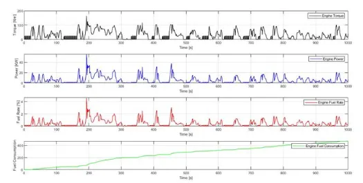
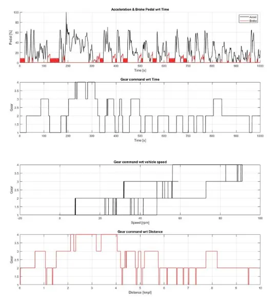
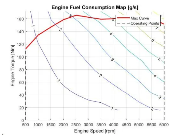
Plots for HWFET cycle
Conclusion
UDDS and HWFET are analysed