Project 2
“Project2_InitFile.m” is a Matlab script used to load all the variables required for running the Simulink model and for post-processing. The drive cycle selection is also done here. Before running the Simulink vehicle model, run this initialization script.
Task:
The task of this project is to quantify the improvement in fuel economy numbers for the hybrid vehicle (kmpl), compared to the conventional vehicle, on the urban cycle (UDDS) and highway cycle (HWFET). Also, to analyze and understand the vehicle operating points in terms of engine and motor speed, torque, transmission speeds, pedal positions, gear, distance traveled, battery voltage, current, SoC etc.
To do that, the following steps need to be followed:
1) Load the Project2 folder as the Current Folder in Matlab.
2) Run the “Project2_InitFile.m” Matlab script.
3) Copy the Conventional vehicle Simulink model created for Project 1 in this folder. Figure 1: P1 Hybrid ArchitectureHybrid Drives Development
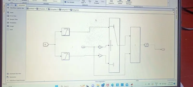
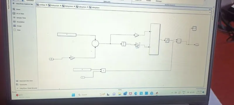
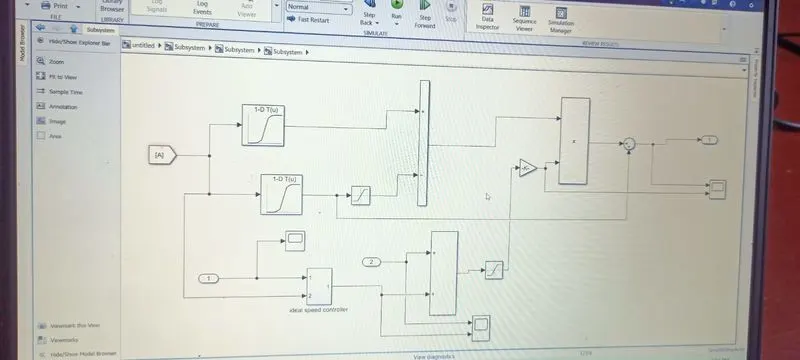
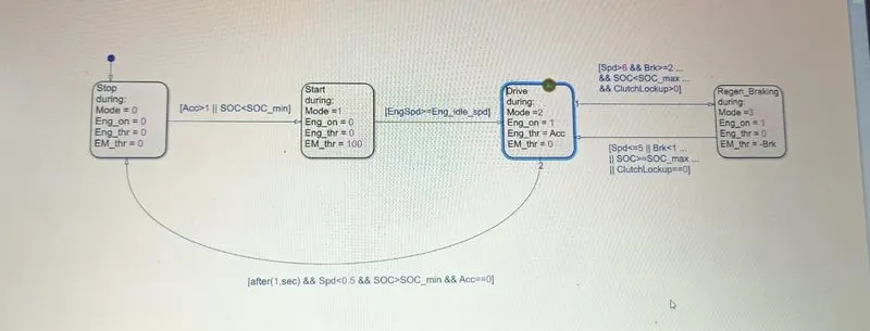
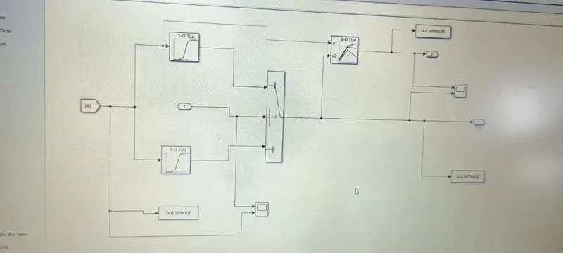
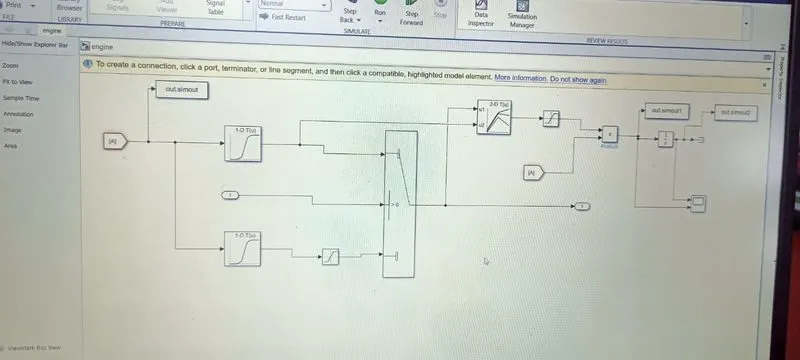
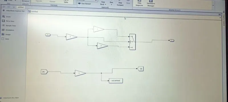
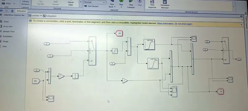
4) Modify this model into a hybrid vehicle model. The lecture presentations can be used as reference. Battery and Supervisory controller models developed in the assignments can be reused.
5) Add additional ‘To Workspace’ blocks for transferring the desired Simulink vehicle data into the Matlab workspace.
6) Simulate the hybrid model on the desired drive cycles.
7) Write a project report that contains the following:
a. Tabulate the fuel economy numbers (kmpl) for UDDS and HWFET cycle. Compare these numbers with the baseline numbers for conventional vehicle model from Project 1.
b. Plot the time trace for engine, transmission input, transmission output and wheel speed on one plot.
c. Plot engine torque, engine power, fuel rate and fuel consumption using subplots.
d. Plot accelerator and brake pedal, gear command, vehicle desired and actual speed, vehicle distance using subplots.
e. Plot the engine operating points on the engine fuel map.
f. Plot motor speed, torque, motor input power using subplots.
g. Plot pack voltage, current and SoC using subplots.
h. Plot the motor operating points on the motor input power map, with the motor max motoring and generating torque curves.
i. Write down appropriate brief comments on each of these plots, describing the vehicle behavior throughout the drive cycle.
j. Generate the plots for both drive cycles.
ANS)
%%%%%%%%%%%%%%%%%%%%%%%%%%%%%%%%%%%%%%%%%%%%%%%%%%%%%%%%%%%%%%%%%%%%%
%% Skill-Lync -> Hybrid Drives Development
% Project 1 - Conventional Vehicle Model
% By - Guruprasad Joshi
%% Post-Processing File
% File for post-processing the Conventional vehicle simulation model data
%% Renaming variables
Time=out.tout;
Acc_Pdl=out.Acc_Pdl; % Accelerator pedal [%]
Brk_Pdl=out.Brk_Pdl; % Brake pedal [%]
Gear_Cmd=out.Gear_Cmd; % Transmission gear
Trans_In_Spd=out.Trans_In_Spd*30/pi; % Transmission input speed [rpm]
Trans_Out_Spd=out.Trans_Out_Spd*30/pi;% Transmission output speed [rpm]
Eng_Trq=out.Eng_Trq; % Engine brake torque [Nm]
Eng_Spd=out.Eng_Spd*30/pi; % Engine speed [rpm]
Eng_Fuel_Consump=out.Eng_Fuel_Consumption; % Engine fuel consumption [g]
Veh_Dist=out.Veh_Dist/1000; % Distance traveled by vehicle [km]
Veh_Spd=out.Veh_Spd*18/5; % Vehicle speed [kmph]
Wheel_Speed=out.Wh_Speed; % Wheel speed [kmph]
Eng_Fuel_Rate=out.Eng_Fuel_Rate % Engine fuel rate [%]
ElecPwr=out.ElecPwr;
EM_Trq=out.EM_Trq;
EM_Spd=out.EM_Spd;
%% Data Analysis
Eng_Pwr=Eng_Spd*(pi/30).*(Eng_Trq/1000); % Engine brake power [kW]
rho_petrol=0.7197; % Density of petrol [kg/L]
%kmpl=Veh_Dist/(Eng_Fuel_Consump/1000/rho_petrol); % Fuel economy [kmpl]
%% Plotting vehicle characteristics time trace
figure(1)
subplot(411)
hold on
grid on
plot(Time,Acc_Pdl);
ylabel('Pedal [%]');
xlabel('Time [s]');
legend('Accel');
subplot(412)
plot(Time,Brk_Pdl);
ylabel('Brk Pedal [%]')
xlabel('Time [s]');
legend('Brake');
subplot(413)
hold on
grid on
plot(Time,Gear_Cmd);
xlabel('Time [s]');
ylabel('Gear');
legend('Gear');
subplot(414)
hold on
grid on
plot(Time,Veh_Dist);
xlabel('Time [s]');
ylabel('Veh_Dist[KM]');
legend('Veh_Dist');
figure(2)
subplot(311)
hold on
grid on
plot(Time,Trans_In_Spd);
ylabel('Speed [rpm]')
legend('Trans Input');
subplot(312)
plot(Time,Trans_Out_Spd);
ylabel('Speed [rpm]')
legend('Trans Output');
subplot(313)
plot(Time,Wheel_Speed);
ylabel('Speed [rpm]')
xlabel('Time [s]');
legend('Wheel_Speed');
figure(3)
subplot(411)
plot(Time,Eng_Fuel_Consump);
ylabel('Engine fuel[g]')
legend('Eng_Fuel_Consump')
subplot(412)
plot(Time,Eng_Fuel_Rate);
ylabel('Engine fuel rate [%]')
legend('Eng_Fuel_Rate');
subplot(413)
plot(Time,Eng_Trq)
ylabel('Engine brake torque [Nm]')
legend('Eng_Trq');
subplot(414)
plot(Time,Eng_Pwr);
ylabel('Eng_Pwr [KW]')
xlabel('Time [s]');
legend('Eng_Pwr');
%% Plotting engine operating points on engine fuel map
figure('Name','Engine Operating Points');
hold on
grid on
title('Engine Operating Points','fontsize',12);
p1=plot(Eng_map_spd*30/pi,Eng_max_trq,'linewidth',2,'color','r');
p2=line([Eng_map_spd(end)*30/pi Eng_map_spd(end)*30/pi],[0 Eng_max_trq(end)]);
set(p2,'linewidth',1,'linestyle','--','color','k');
p3=line([Eng_map_spd(1)*30/pi Eng_map_spd(1)*30/pi],[0 Eng_max_trq(1)]);
set(p3,'linewidth',1,'linestyle','--','color','k');
[c,h] = contour(Eng_map_spd'*30/pi,Eng_map_trq,Eng_fuel_map');
clabel(c,h);
xlabel('Engine Speed [rpm]');
ylabel('Engine Torque [Nm]');
title('Engine Fuel Consumption Map [g/s]');
p4 = plot(Eng_Spd,Eng_Trq,'.','color','k');
legend([p1 p4],{'Max Curve','Operating Points'});
axis([Eng_map_spd(1)*30/pi Eng_map_spd(end)*30/pi 0 Eng_map_trq(end)]);