Project

BAJA All-Terrain Vehicle (ATV) analy

AIM:

To carry out a system-level simulation of an all-terrain vehicle using Simulink. To prepare a technical report on BAJA ATV explaining model properties for the following:

1. CVT Model without dashboard,
2. CVT Model with dashboard,
3. CVT Model using Lookup table Mapped &
4. CVT Model dashboard Mapped.

THEORY:

ATV: An all-terrain vehicle (ATV) refers to a motorized single­ seated tri or quadric cycle bike and buggy that is designed for off­ road travel and activities. The vehicle consists of handlebars and low-pressure tires that have deep-threaded structures, which assist in driving over muddy, rocky, wetlands and dune topologies. In comparison to other utility vehicles (UTVs). ATVs offer excellent off-road capabilities and can carry heavy equipment over long distances and narrow access points. They can also be customized for high-performance riding, owing to which they find extensive applications across various industries, including sports, entertainment, agriculture, military and defense.

CVT: A CVT or Continuously Variable Transmission is an automatic, single-speed, and gearless transmission that can shift through an infinite number of gear ratios. A continuously variable transmission (CVT) is a transmission that operates on an ingenious pulley system that automatically varies the transmission ratio, allowing an infinite variability between highest and lowest gears with no discrete steps or shifts. CVTs provide more useable power, better fuel economy and smoother driving experience than traditional transmissions that use gearboxes with fixed numbers of gear sets.

Solution:

1. CVT Model Without Dashboard

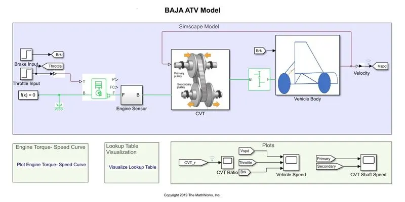
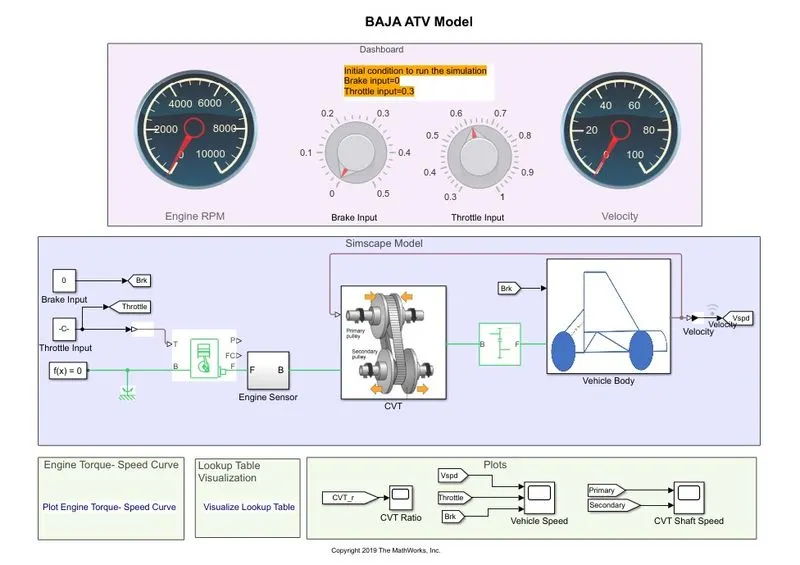
A Simulink model for the BAJA ATV Model is shown below. The models consist of common blocks as follows:

Signal Builder: The Signal Builder block allows you to create interchangeable groups of piecewise linear signal sources and use them in a model. You can quickly switch the signal groups into and out of a model to facilitate testing.

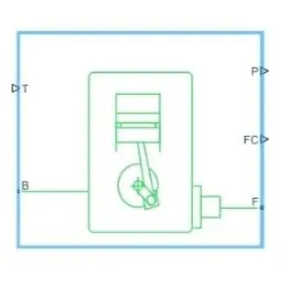
Generic Engine: Represents a system-level model of spark-ignition and diesel engines suitable for use at initial stages of modeling when only the basic parameters are available. Optional idle speed and red line controllers are included. The throttle input signal T lies between zero and one and specifies the torque demanded from the engine as a fraction of the maximum possible torque. If the engine speed falls below the Stall speed, the engine torque is blended to zero. If the engine speed exceeds the maximum speed, the simulation stops and issues an error message. Connections F and B are mechanical rotational conserving ports associated with the engine crankshaft and engine block, respectively. Connections P and FC are physical signal output ports through which engine power and fuel consumption rate are reported. Speed vector and Torque vector are the assigned parameters.

Engine Sensor:

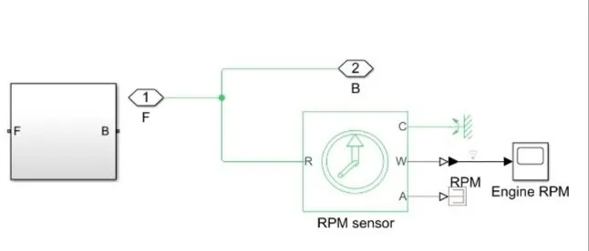
Ideal Rotational Motion Sensor: The block represents an ideal mechanical rotational motion sensor, that is, a device that converts an across variable measured between two mechanical rotational nodes into a control signal proportion all to angular velocity or angle. The sensor is ideal since it does not account for inertia, friction, Delays, energy consumption and so on. Connections R and C are mechanical rotational conserving ports and connections Wand A are physical signal output ports for velocity and angular displacement respectively.

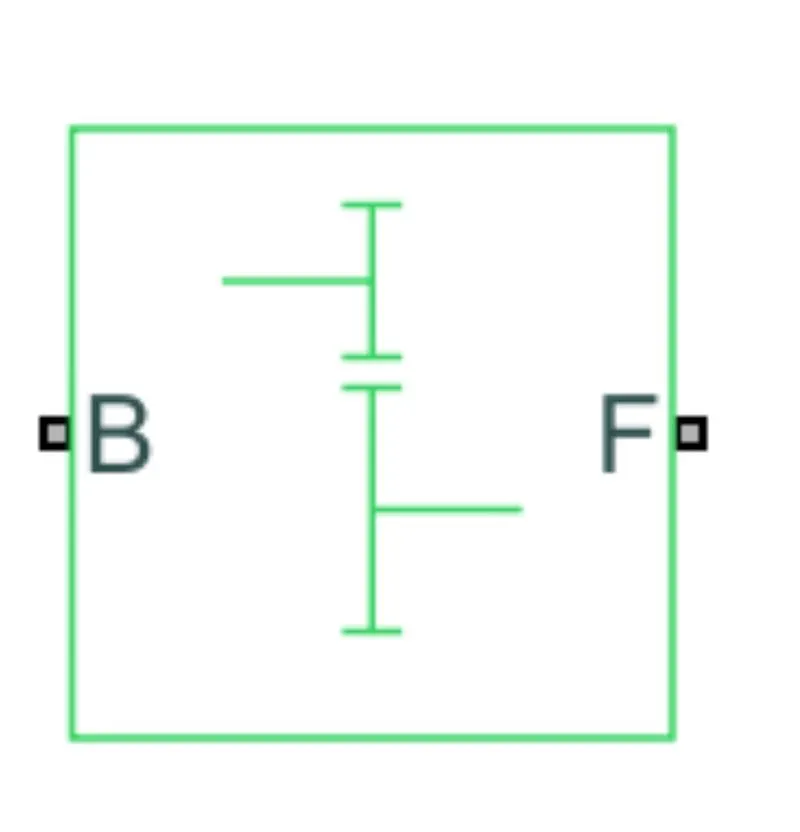
Simple Gear: Represents a fixed-ratio gear or gearbox. No inertia or compliance is modeled in this block. You can optionally include gear meshing and viscous bearing losses. Connections B (base) and F (follower) are mechanical rotational conserving ports. Specify the relation between base and follower rotation directions with the Output shaft rotates parameter. Optionally include thermal effects and expose thermal conserving port H by right-clicking on the block and selecting Simscape block choices to switch between variants.

Gear Ratio= Follower gear speed/Base gear speed

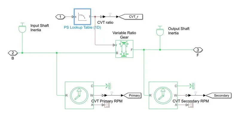
CVT Subsystem:

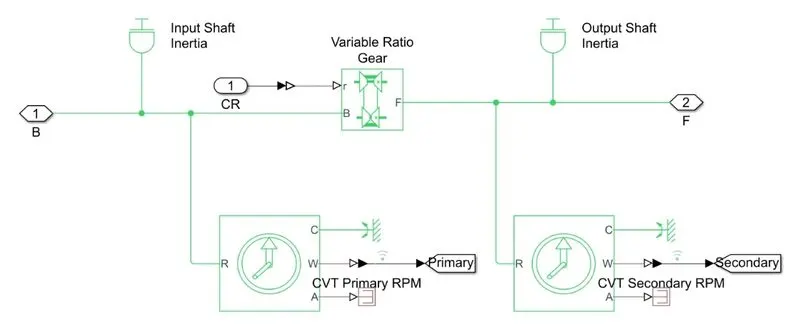
The CVT Subsystem consists of the following blocks:

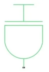
Inertia: The block represents an ideal mechanical rotational inertia. The block has one mechanical rotational conserving port. The block positive direction is from its port to the reference point. This means that the inertia torque is positive if the inertia is accelerated in a positive direction.

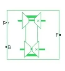
Variable Ratio Transmission: Represents a variable ratio gearbox such as implemented by mechanical belt CVT, electric, or hydraulic transmissions. The physical signal input r defines the ratio of input to output angular shaft velocities. Connections B (base) and F (follower) are mechanical rotational conserving ports. Specify the relation between base and follower rotation directions with the Output shaft rotates parameter.

Vehicle Body Subsystem:

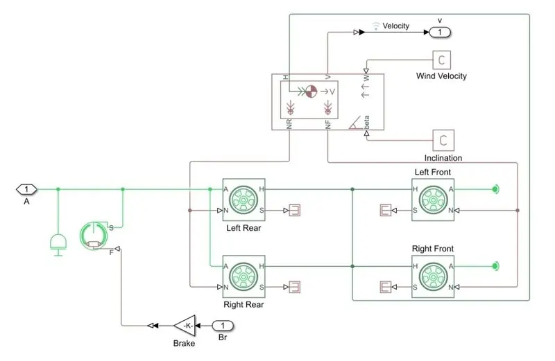
The Vehicle Body Subsystem consists of the following blocks:

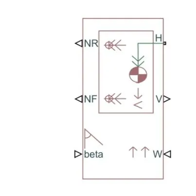
Vehicle Body: Represents a two-axle vehicle body in longitudinal motion. The block accounts for body mass. aerodynamic drag, road incline and weight distribution between axles due to acceleration and road profile. The vehicle can have the same or a different number of wheels on each axle. Optionally include pitch and suspension dynamics or additional variable mass and inertia. The vehicle does not move vertically relative to the ground. Connection H is the mechanical translational conserving port associated with the horizontal motion of the vehicle body. The resulting traction motion developed by tires should be connected to this port. Connections V, NF and NR are physical signal output ports for vehicle velocity and front and rear normal wheel forces, respectively. Wheel forces are considered positive if acting downwards. Connections Wand beta are physical signal input ports corresponding to headwind speed and road inclination angle, respectively. If the variable mass is modeled, the physical signal input ports CG and M are exposed. CG accepts a two-element vector representing the x and y distance offsets from vehicle CG to additional load mass CG. M represents the additional mass. If both variable mass and pitch dynamics are included the physical signal port J accepts the inertia of the additional mass about its own CG.

Parameters are: Mass: 250 kg, Number of wheels per axle: 2, Horizontal distance from CG to front axle: 1m, Horizontal distance from CG to rear axle: 0.35 m, CG height above ground: 0.7 m, Gravitational acceleration: 9.81 m/s2

Tire: Represents the longitudinal behavior of a highway tire characterized by the tire Magic Formula. The block is built from Tire-Road Interaction (Magic Formula) and Simscape Foundation Library Wheel and Axle blocks. Optionally, the effects of tire inertia, stiffness and damping can be included. Connection A is the mechanical rotational conserving port for the wheel axle. Connection H is the mechanical translational conserving port for the wheel hub through which the thrust developed by the tire is applied to the vehicle. Connection N is a physical signal input port that applies the normal force acting on the tire. The force is considered positive if it acts downwards. Connection Sis a physical signal output port that reports the tire slip. Optionally expose physical signal port M by setting Parameterize by to Physical signal Magic Formula coefficients. Physical signal port M accepts a four-element vector corresponding to the B. C, D, and E Magic Formula coefficients.

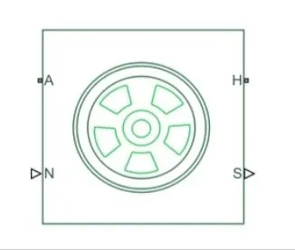
Parameterize by: Constant Magic Formula coefficients Magic Formula B coefficient: 10 Magic Formula C coefficient: 1.9 Magic Formula D coefficient: 1 Magic Formula E coefficient: 0.97

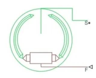
Double-Shoe Brake: Represents a brake arranged as two pivoted rigid shoes symmetrically installed inside or outside a drum and operated by one actuator. The actuator force causes the shoes to exert a friction torque on a shaft connected to the drum. Connection Sis a conserving rotational terminal associated with the drum shaft. Connection F is a physical signal port representing the force input to the actuator. Positive force creates friction torque that resists shaft rotation. Optionally include thermal effects and expose thermal conserving port H by setting Thermal port to Model.

Parameters are: Drum radius: 150 mm, Actuator location radius: 100 mm, Pin location radius: 125 mm, Pin location angle: 15deg, Shoe beginning angle: 5 deg, Shoe span angle: 120 deg

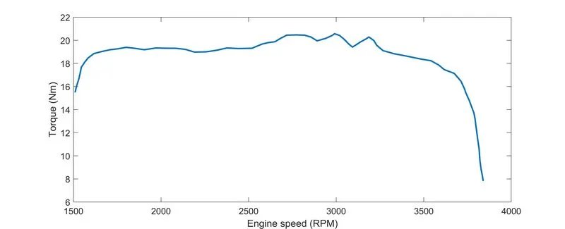
Torque vs Speed Characteristics:

Process:

a) Throttle signal and break signal generated by signal builder block, these two signals are given as input to generic engine.

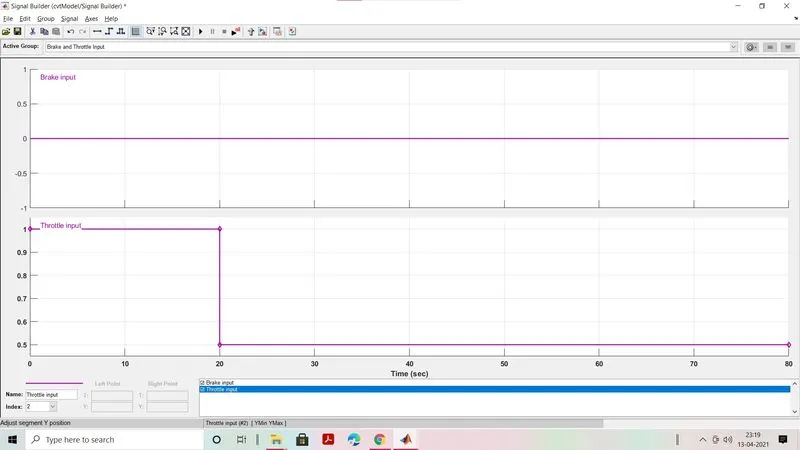
b) Torque and Speed vector inputs are taken from Matlab workspace.

c) Generic Engine will generate the output RPM that can be taken from the crankshaft output. This RPM speed is given as input to the Ideal Rotational Sensor to sense the output RPM from shaft, this same output is given to the simple gear mechanism to reduce the speed where the gear ratio is 10.

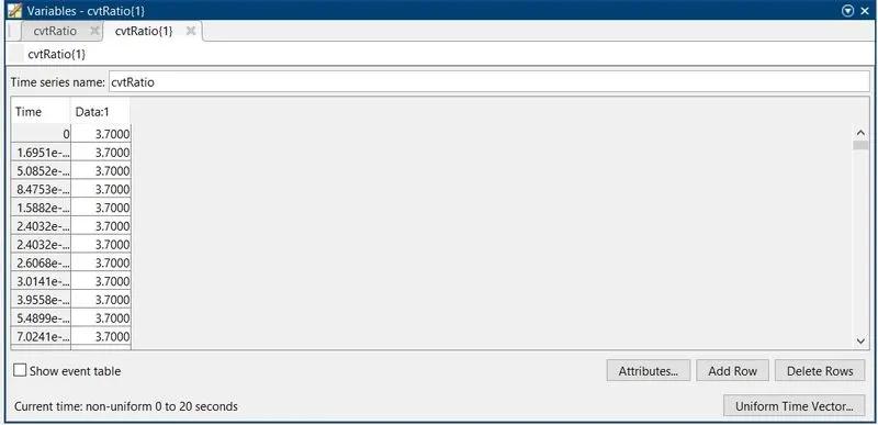
d) Output from the sensor and ratio through the signal builder given as input to the CVT block (Variable Ratio Transmission).

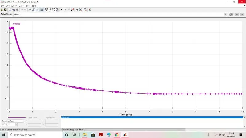
e) Speed is controlled by the variable CVT ratios and this controlled output speed is given input to the vehicle axle.

f) Power from the CVT is input to the axle then the vehicle accelerates according to the speed.

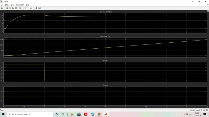
g) Output from the Vehicle body is taken as Velocity.

Result:

Torque - Speed characteristics

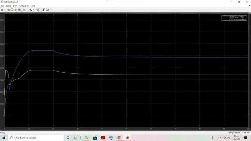
CVT Shaft Speed Plot

Engine RPM

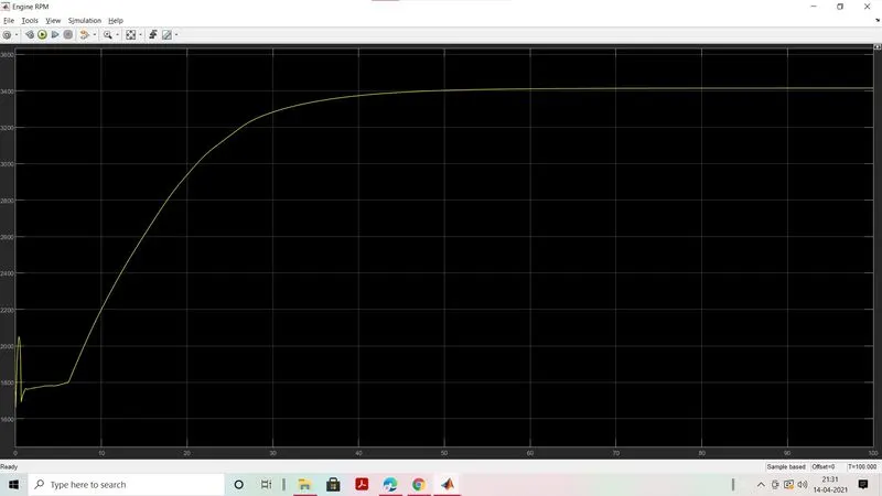
here in this plot we cn see the engine RPM generated according to the speed, throttle & torque.

2. CTV Model With Dashboard

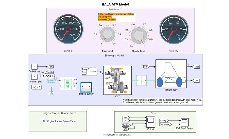
Main Model:

Dashboard:

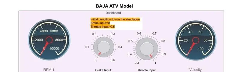
The above model workflow process is same as the model without dashboard but the brake and throttle inputs are controlled by Knob.

Results:-

Inputs to the CVT

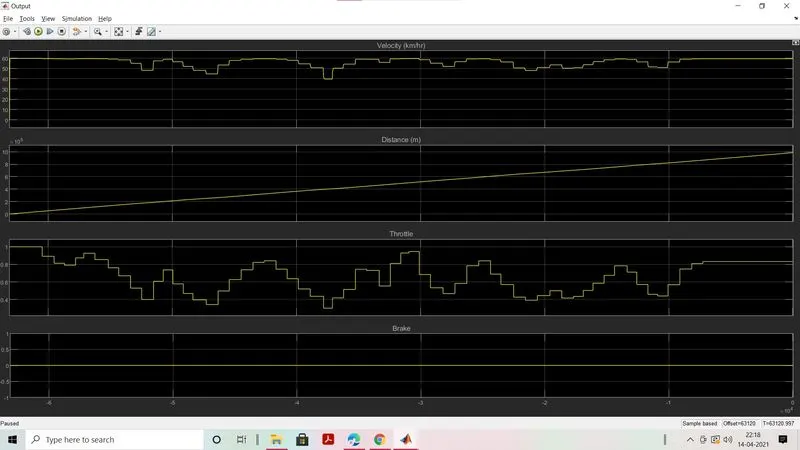
Runtime is defined by the Knob rotation

Engine Speed Plot,

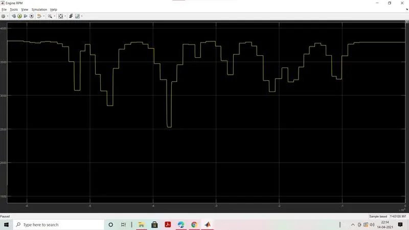
Here the engine speed is generated according to the inputs throttle, brake, torque and speed vectors.

CVT Shaft Speed plot,

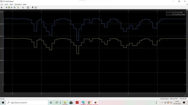
step up and step down are acceleration and deceleration respectively. the linear one is the constant speedd so no changes in throttle or braking.

3. CVT Model using Lookup table Mapped:

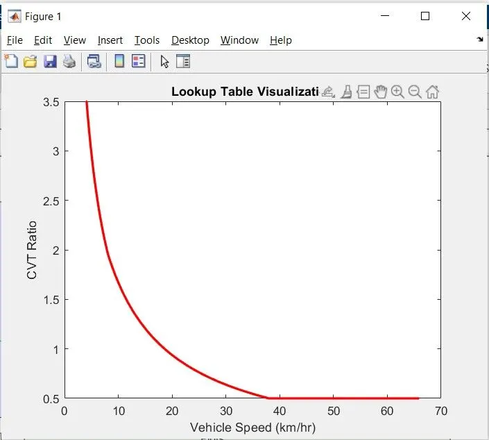
Lookup table 1D: This block represents a physical signal converter whose input-output relationship is specified by a lookup table. The table grid must be in strictly ascending or strictly descending order, but the spacing can be nonuniform. Right-click on the block and select Foundation Library > Plot Table to visualize the table data based on the selected interpolation and extrapolation methods. This block does not propagate physical signal units and will be removed in a future release.

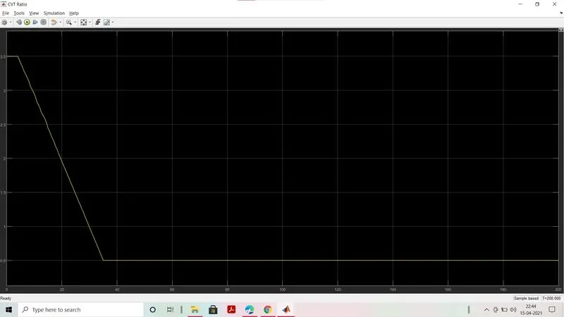
CVT Ratio vs Vehicle speed:

Output:

CVT Shaft Speed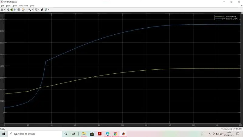

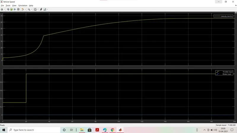
Vehicle Speed

Lookup table Visualization

4. CVT Model with dashboard Mapped:

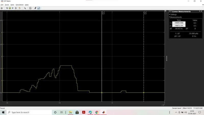
CVT Ratio:

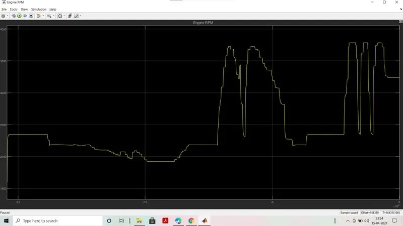
Engine RPM:

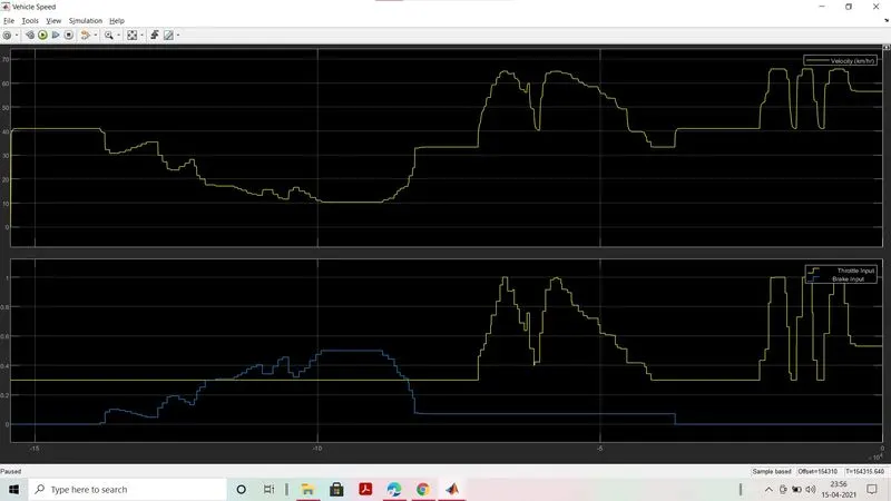
Vehicle Speed:

CVT Shaft Speed: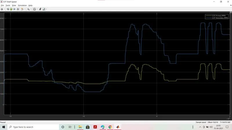

Observations:

a) CVT Shaft speed, Velocity and Engine speed are directy proportional to the Throttle input and inversely proportional to the Brake input.

b) CVT Ratio is directly proportional to Torque and inversely proportional to the Throttle input.

c) CVT Primary speed is greater than Secondary speed as they are directly proportional to their shaft diameter.

d) The speed might get null at a particular breaking resistance.