Week 3 - Solving second order ODEs

Objective:

The Main objective of this project is to simulate the transient behaviour of the simple pendulum and to create animation of its motion using Matlab program by solving the second order ODE.

Simple Pendulum:

A simple pendulum consists of a mass (M) hanging at the end of a string of length (L).

The period of a pendulum or any oscillatory motion is the time required for one complete cycle, i.e.; the time to go back and forth once. If the amplitude of motion of the swinging pendulum is small, then the pendulum behaves approximately as a simple harmonic oscillator, and the period T of the pendulum is given by T=2*`pi``root`(l/g)

Simple Harmonic motion:

In mechanics and physics, simple harmonic motion is a special type of periodic motion or oscillation where the restoring force is directly proportional to the displacement and acts in the direction opposite to that of displacement.

The motion of a particle moving along a straight line with an acceleration whose direction isalways towards a fixed point on the line and whose magnitude is proportional to the distance from the fixed point is called simple harmonic motion.

By applying Newton's second Law of rotational motion, we can get the equation of motion for the pendulum with damping co-efficient is d/dt^2(`theta`)+(b/m)*d/dt(`theta`)+(g/l)*sin`theta` = 0

in the above equation,

g = gravity in m/s^2,

l = length of the pendulum in m,

m = mass of the ball in kg,

b = damping co-efficient.

Now, for solving these kind of higher order ODE, we can break the equation into first order ODE.

Let us consider `theta` = `theta`1

Then d/dt(`theta`) = d/dt(`theta1`) = `theta2` this is equation 1`

d^2/dt^2 `theta` = d^2 `theta1`/dt^2

`\Rightarrow`d/dt*(`theta`2) this is equation 2.

substituting `theta` = `theta1` in original equation

d^2 `theta1`/dt^2 + b/m(d`theta1`/dt) +g/l(sin`theta1`) = 0,

Then substituting equation 1 & 2

`d theta2`/dt + b/m(`theta2`) + g/l(sin`theta1`) = 0

`d theta2`/dt = -b/m(`theta2`) - g/l(sin`theta1`)

d/dt`[(theta1),(theta2)]` = `[(theta2),((-b/m).theta2-(g/l).sintheta1)]`

the above equation is the solution vector in the form of matrix.

let us assume the input parameters as follows;

l = 1 meter,

m = 1kg,

b = 0.05,

g = 9.81 (m/s)^2,

time = 0-20 sec in simulation

angular displacement = 0,

angular velocity = 3 rad/sec.

Architecture for this program is like

1. Input parameters: Here we require input parameters like length of string, mass of the bob, damping coefficient and acceleration due to gravity.

2. Initial conditions and time period: here we are defining the initial conditions like angular displace ment and angular velocity in the form of array into a new variable called thera_0. then the time period for the oscilations is declared with the help of linespace command from 0 to 20 with 200 points and assinging it to the variable called time_span.

3. Function ODE45: In this step we are solving the ODE equation with the help of inbuilt ODE solver command in Matlab.

%solving ODE

[t,results] = ode45(@(t,theta)ode_func(t,theta,b,g,l,m,time_span,theta_0);

Here we first defining ode45 is the function of t and theta, because these 't' & 'theta' is only the dependent and independent variable of the ode system. Then we are calling our theta_0 is initial condition.

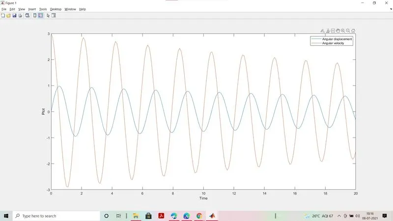
4. Plotting graph: Here we are plotting the graph which shows the angular displacement and the angular velocity wth respect to the time period of oscilliation. we can observe the changes in the graph b changing the damping coefficient also.

5. Creating Animation with for loop: Here in for loop we declaring the value with the range operator to the length of the result value 1, which is nothing but the angular displacement values. Then we are assigning into the new variable called (i). Next process is to give the co-ordinates value for the string where the ball is hanging. X0,Y0 & X1,Y1 are the variables which store the values for string.

6. Plotting the figure under loop: During plotting under the for lopp, we are plotting the horizontal line with red and vertical line which is our string green in color. The ball is plotted at the end of the string with the help of marker and the marker size and face color is also declared.

7. Creating the video file: Finally we created the video file with the help of getframe, loop counter, video writer and open video, close video commands.

Main Program in Matlab:

% Program to solve Second Order Differential equation

close all
clear all
clc

% Input Parameters for the given equation
l = 1;
Ma = 1;
b = 0.05;
g = 9.81;

% Initial Condition
theta_0 = [0;3];

% Time points
time_span = linspace(0,20,200);

% Solving ODE
[t,results] = ode45(@(t,theta) ode_func1(t,theta,b,g,l,Ma),time_span,theta_0);

% Plotting
figure(1)
plot(t,results(:,1));
hold on
plot(t,results(:,2));
xlabel('Time');
ylabel('Plot');

legend('Angular displacement','Angular velocity');

% Creating Animation
ct = 1;
for i = 1:length(results(:,1))
    x0 = 0;
    y0 = 0;
    
    x1 = 1*sin(results(i,1));
    y1 = -1*cos(results(i,1));
    
    figure(2)
    plot([-1.5,1.5],[0,0],'linewidth',3,'color','r');
    hold on
    plot([x0 x1],[y0 y1],'linewidth',1,'color','g');
    plot(x1,y1,'marker','o','markerface','b','markersize',15);
    axis([-2,2,-2,2]);
    title('Simple Pendulum Oscillation');
    pause(0.1);    
    M(ct) = getframe(gcf);
    ct = ct+1;
    hold off
end

movie(M)
videofile = VideoWriter('simple_pendulum.avi','uncompressed AVI');
open(videofile)
writeVideo(videofile,M)
close(videofile)
    

Function Code:

Function is set of command used to perform the task. The main purpose of the function command we can run this with any set of values when needed. This will reduce the main program size. In matlab the function name and the function file should be stored in the same name as well as in the same path.

Code:

% function of time and theta

function  [dtheta_dt] = ode_func1(t,theta,b,g,l,Ma)
theta1 = theta(1);
theta2 = theta(2);
dtheta1_dt = theta2;
dtheta2_dt = (-b/Ma)*theta2-(g/l)*sin(theta1);
dtheta_dt = [dtheta1_dt; dtheta2_dt];
end

in the above function command ode_func is the function name with the set of input values which will be declared in the main program. Then we are storing the output with the new variable name called [dtheta_dt]. The array bracket is used since we are going to get the output in the form of colomn array.

Plotting Figure:

Result: Video of Simple Pendulum

https://youtu.be/QUPN5XVNI6c