System-level simulation for all terrian vehicle.

Aim: To carry out a system-level simulation of all-terrain vehicle

Objective:

• To prepare the technical report by explaning the model properties and comment on the result.
• To study all the 4 models of simulink (i.e open loop,closed loop,mapped model using lookup table).

Theory: An all-terrain vehicle (ATV), also known as a light utility vehicle (LUV), a quad bike, or simply a quad, as defined by the american national standard intitute(ANSI); is a vehicle that travels on low-pressure tires, with a seat that is straddled by the operator, along with handlebars for steering control. As the name implies, it is designed to handle a wider variety of terrain than most other vehicles

Baja SAE is an Collegiate design series competition run by the Society of Automotive Engineers International (SAE International). Teams of students from universities all over the world design and build small off-road cars. The cars all have engines of the same specifications. As of 2018 the engine has been an unmodified Model 19 Vanguard engine single-cylinder with a displacement of 305cc and power output of approximately 10 bhp (7.5 kW).

Baja SAE is an intercollegiate engineering design competition for undergraduate and graduate engineering students. The object of the competition is to simulate real-world engineering design projects and their related challenges. Each team is competing to have its design accepted for manufacture by a fictitious firm. The students must function as a team to design, build, test, promote and compete a vehicle within the limits of the rules, also to generate financial support for their project and manage their educational priorities.

Each team's goal is to design and build a prototype of a rugged, single seat, off-road recreational vehicle intended for sale to the non-professional weekend off-road enthusiast. The vehicle must be safe, easily transported, easily maintained and fun to drive. It should be able to negotiate rough terrain without damage. As of 2010, the SAE Baja Series consisted of three competitions, though in the past there have been as many as seven sanctioned events. A Baja SAE competition event consists of three to four days.

Important blocks used in simscape models which are as follows:

1. CVT
2. VEHICLE BODY
3. GENERIC ENGINE
4. SIMPLE GEARS
5. DOUBLE SHOE BRAKE

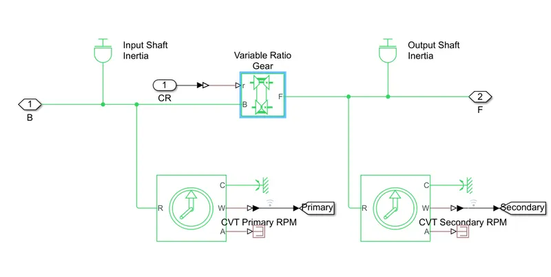
1-CVT(continuously variable transmission)

A continuously variable transmission (CVT) is an automatic transmission that can change seamlessly through a continuous range of gear ratios. This contrasts with other transmissions that provide a limited number of gear ratios in fixed steps. The flexibility of a CVT with suitable control may allow the engine to operate at a constant RPM while the vehicle moves at varying speeds.

The most common type of CVT uses two pulleys connected by a belt or chain, however, several other designs have also been used at times.

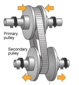
A CVT is a transmission having a speed ratio that can be varied continuously over its allowable range. Its speed ratio may take on any value between its operational limits, i.e., an infinite number of ratios are possible. A gearbox transmission, on the other hand, has a discrete number of fixed speed ratios.

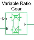
Where, B and F = rotational conserving ports

The Variable Ratio Transmission block represents a gearbox that dynamically transfers motion and torque between the two connected driveshaft axes, base and follower.

Ignoring the dynamics of transmission compliance, the driveshafts are constrained to corotate with a variable gear ratio that you control. You can choose whether the follower axis rotates in the same or opposite direction as the base axis. If they rotate in the same direction, ω_Fand ω_B have the same sign. If they rotate in opposite directions, ω_F and ω_B have opposite signs.

Transmission compliance introduces internal time delay between the axis motions. Therefore, unlike a gear, a variable ratio transmission does not act as a kinematic constraint. You can also control torque loss caused by transmission and viscous losses

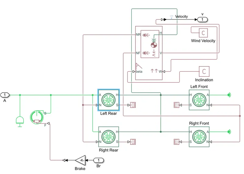
2-Vehicle body:

The Vehicle Body block represents a two-axle vehicle body in longitudinal motion. The vehicle can have the same or a different number of wheels on each axle. For example, two wheels on the front axle and one wheel on the rear axle. The vehicle wheels are assumed identical in size. The vehicle can also have a center of gravity (CG) that is at or below the plane of travel.

The block accounts for body mass, aerodynamic drag, road incline, and weight distribution between axles due to acceleration and road profile. Optionally include pitch and suspension dynamics. The vehicle does not move vertically relative to the ground.

The block has an option to include an externally-defined mass and an externally-defined inertia. The mass, inertia, and center of gravity of the vehicle body can vary over the course of simulation in response to system changes.

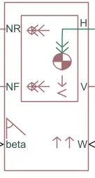
where,W = Headwind speed(m/s)

beta = Road incline angle(rad)

H = Horizontal motion

V = Longitudinal velocity(m/s)

NR = Rear axle normal force(N)

NF = Front axle normal force(N)

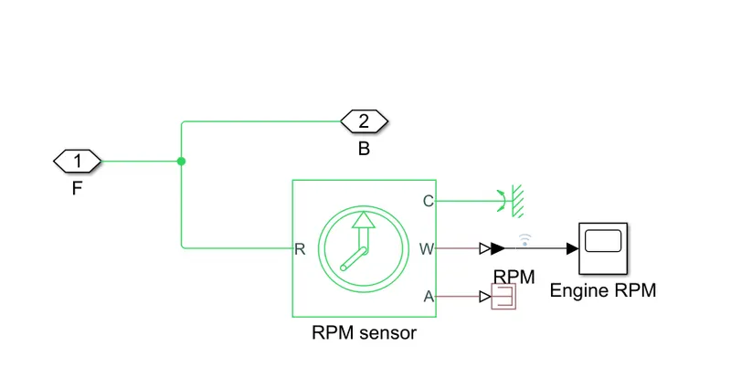
3-Generic Engine:

The Generic Engine block represents a general internal combustion engine. Engine types include spark-ignition and diesel. Speed-power and speed-torque parameterizations are provided. A throttle physical signal input specifies the normalized engine torque. Optional dynamic parameters include crankshaft inertia and response time lag. A physical signal port outputs engine fuel consumption rate based on choice of fuel consumption model. Optional speed and redline controllers prevent engine stall and enable cruise control.

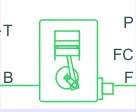
Where,T = Physical signal input port specifying the normalized engine throttle level

B = Rotational conserving port representing the engine block

P = Physical signal output port reporting the instantaneous engine power, in W

FC = Physical signal output port reporting the fuel consumption rate, in kg/s

F = Rotational Conserving port representing the engine crankshaft

4-Simple Gears:

The Simple Gear block represents a gearbox that constrains the connected driveline axes of the base gear, B, and the follower gear, F, to corotate with a fixed ratio that you specify. You choose whether the follower axis rotates in the same or opposite direction as the base axis. If they rotate in the same direction, the angular velocity of the follower, ω_F, and the angular velocity of the base, ω_B, have the same sign. If they rotate in opposite directions, ω_F and ω_B have opposite signs.

Where, B and F are base and followers

5-Double shoe brake:

The Double-Shoe Brake block represents a frictional brake with two pivoted rigid shoes that press against a rotating drum to produce a braking action. The rigid shoes sit inside or outside the rotating drum in a diametrically opposed configuration. A positive actuating force causes the rigid shoes to press against the rotating drum. Viscous and contact friction between the drum and the rigid shoe surfaces cause the rotating drum to decelerate.

Double-shoe brakes provide high braking torque with small actuator deflections in applications that include motor vehicles and some heavy machinery. The model employs a simple parameterization with readily accessible brake geometry and friction parameters.

You can also enable faulting. When faulting occurs, the belt will exert a user-specified force. Faults can occur at a specified time or due to an external trigger at port T.

Where, S = Drum shaft rotation

F = Actuating force

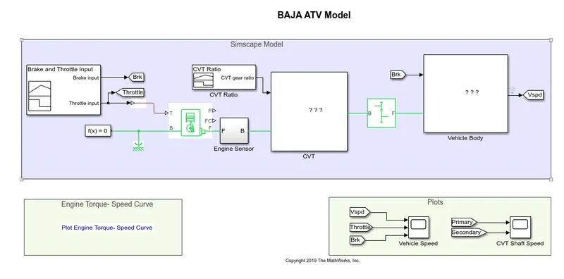
1- Simulink model of baja model without dashboard :

Simulink model:

SUB-BLOCKS:

CVT BLOCK:

Vehicle body block:

Engine sensor block:

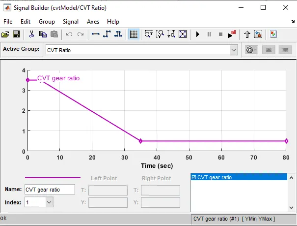
• Here we used 2 seprate signal builder blocks each one for brake &throttle input and another block for CVT gear ratio.

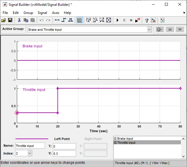
• From this signal builder we can understand that the input for brake is always zero for all conditions and the throttle input is 0.3 upto 20 sec of time and then its been increased to 1 and kept constant upto 80 sec.
• Below signal builder block is for CVT gear ratios and by looking at that plot we can see that the input which we gave is 3.5 initially at 0 sec and this is gradually decreasing to 0.5till 35 sec after 35 sec the gear ratio is kept constant upto 80 sec which 0.5.

Output:

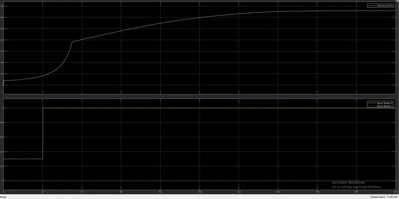
• In output first by observing the first plot we observe that how the velocity is increasing, at initial throttle value upto 35 s the velocity is increaing in parabolaic curve in nature and and after that its starts increasing in continuous manner without and discontinuity and after 140 it is seen that velcity is constant 68kmph till endrun time i.e 200sec

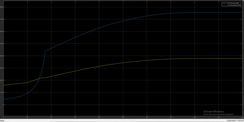
• Here by looking at plot the primary cvt at initial throttle value upto 20 sec it seems to be increasing lineraly and after increasing throttle value from 0.5 to 1 there some deviations in rpm upto 38 sec and after 40 sec rpm is been seen linearly increasing at constant throttle.
• In secondary cvt at output shaft it is been seen that the input throttle given to variable gear ratios its increasing with some losses and after some time i.e 140 s the cvt values matches with primary cvt which is constant till 200sec.

2-Simulink model of baja with dashboard:

Simulink model:

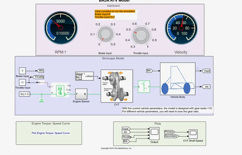
Explanation:

• In simscape model instead of the signal bulider block we used is the dashboard with two knobs of brake and throttle in which we gave the input as for brake input is 0 and throttle is 0.5 and we plot the reult for inf ti,e and stoped the run time at some point and visualize the result.
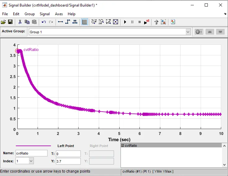
• Below shown is the cvt signal builder block in which we can see that at 0 the ratio was 3.7 initially and after some time with respect to time the ratio starts decreasing and after 6 s the ratio was constant throughout at 0.7.

Output:

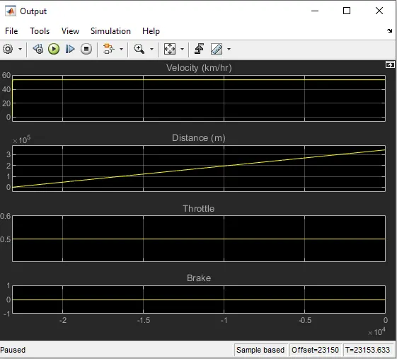
As we can see that after giving input of brake as 0 and throttle value as 0.5 constant throughout the speed as the vehichle is moving at 58kmph with a constant speed with linear increasing in a distance.

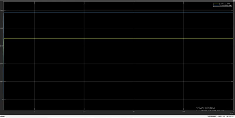
• After observing the output for primary and secondary cvt rpm it is oerved that primary cvt rpm started increasing after giving thrrotle upto 3400rpm amd after that rpm was constant throughout with respect tp chnage in velocity and time.
• Secondary cvt rpm is in increasing manner for intiall throttle value and it attined 4800 rpm and after that with respect to time and velocity it was constant .

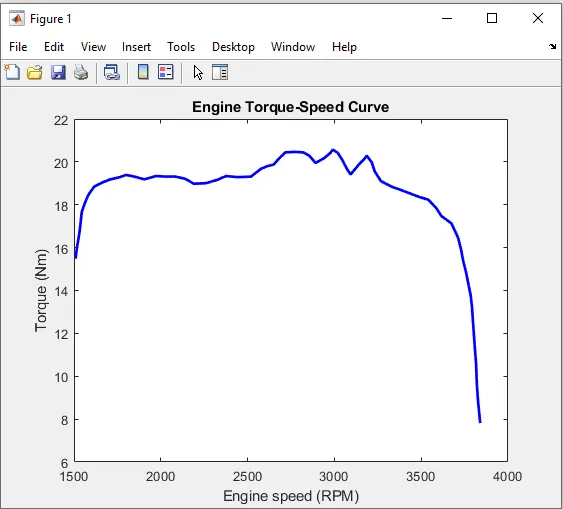
Below we can see the plot of vehicle torque vs Rpm as it is observed that there is uneven cnahge in torque as the rpm changes after 3000 rpm torque value seems to be descreasing from 18Nm to 8Nm, as we know if speed increases torque decreases and vice versa.

3-Simulink model without dashboard but using lookup table for input values:

Simulink model:

Explanation:

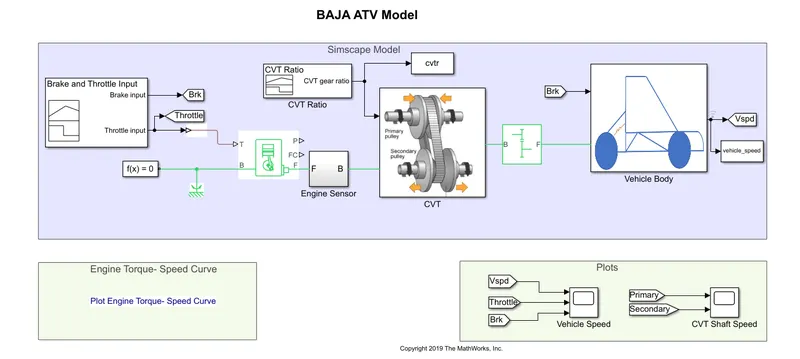
• Here we used the lookup table to visualize the results.Lookuptable is the array of data which is used to map the input values to output values.
• In other words the lookup table computes the mathematical function of the model i.e y=f(x).
• We used this lookup table to give the input values as cvt and vehcle speed and maped out the reults.
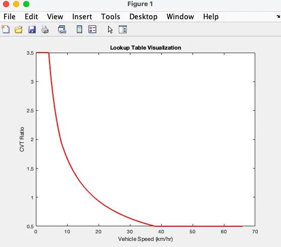
• Below we can see the lookup table plot according to which we gave as input values as initially the cvt ratio was 3.5 upto some 5-6 kmph speed and after that with increasing speed the cvt ratio starts decreasing and cvt ratio became 0 after speed was 38kmph and throughout the cvt was 0 for vehicle spee ahead.
• From this signal builder we can understand that the input for brake is always zero for all conditions and the throttle input is 0.3 upto 20 sec of time and then its been increased to 1 and kept constant upto 80 sec.
• Below signal builder block is for CVT gear ratios and by looking at that plot we can see that the input which we gave is 3.5 initially at 0 sec and this is gradually decreasing to 0.5till 35 sec after 35 sec the gear ratio is kept constant upto 80 sec which 0.5.

Output:

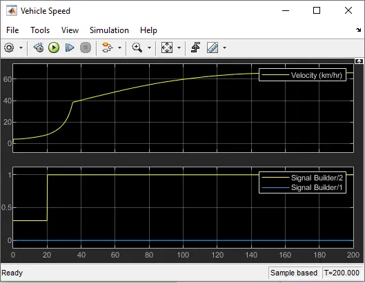
• After using the lookup table input values we observe that the velocity initially started increasing from 0 to 3.5 after that as the cvt ratio was in decreasing manner by increasing in speed we can observe here in plot the curve which is parablic form and afte some time when cvt value is zero velocity was constant and this plot also the after some time speed is linearlyincreasing manner and after some time it attains linearity without any varies in speed.

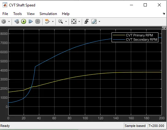
• Here by looking at plot the primary cvt at initial throttle value upto 20 sec it seems to be increasing lineraly and after increasing throttle value from 0.5 to 1 there some deviations in rpm upto 38 sec and after 40 sec rpm is been seen linearly increasing at constant throttle.
• In secondary cvt at output shaft it is been seen that the input throttle given to variable gear ratios its increasing with some losses and after some time i.e 140 s the cvt values matches with primary cvt which is constant till 200sec.

4-Simulink model with dashboard and using lookup tables for input values:

Simulink model:

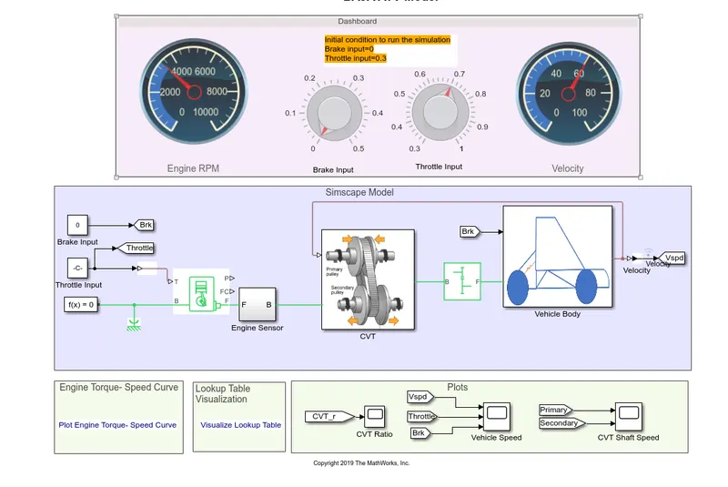
Explanation:

• Here we used the lookup table for input values for cvt ratio and vehicle speed and through knob we changed the throttle values to 0.7 and brake input is kept at zero.
• Lookuptable is the array of data which is used to map the input values to output values.
• In other words the lookup table computes the mathematical function of the model i.e y=f(x).
• We used this lookup table to give the input values as cvt and vehcle speed and maped out the reults.

Output:

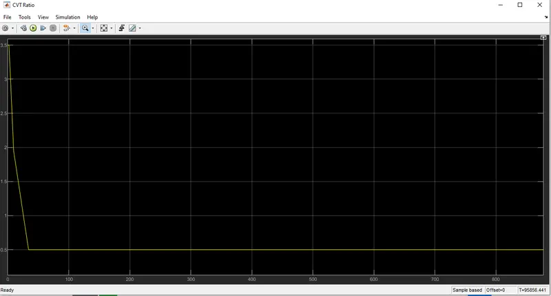
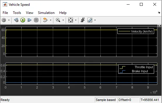
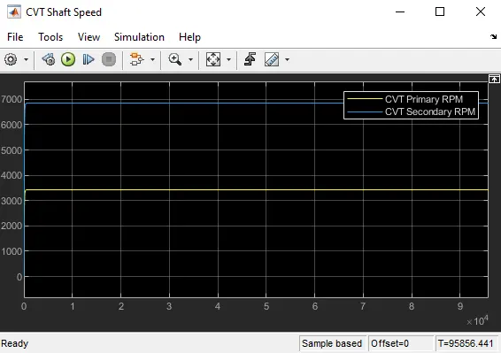
• Here by observing cvt ratio plot we see that initiall the ratio was 3.5 and after that it started dercreasing with respect to increase in speed and was constant at 0.5 after 60kmph speed of the vehicle.
• Here by observing vehicle speed plot speed was not linear for some time with decreasing cvt ratio after that it attended the linear speed as the cvt ratio became constant at 0.5 and throttle was kept constant at 0.7.
• In secondary and primary cvt rpm at input shaft primary cvt rpm was increasing in non linear manner upto 3500 rpm and after that as the cvt ratio got constant the input shaft rpm became constant and same as for secondary cvt rpm the rpm at output shaft after cvt ratio became constant the rpm was 6800 rpm and was constant throughout.

Conculsion:

We studied all the conditions of baja atv where we used lookup table for 2 conditions and for 2 conditions we manually changed the values by changing parameters and knob values and ploted the results.