Project

OBJECTIVES OF THE PROJECT

1. To Prepare a technical report explaining the model properties & comments on the results
2. Explain the functions of the subsystems & blocks used for preparing the model

BAJA All-Terrain Vehicle (ATV) Models:

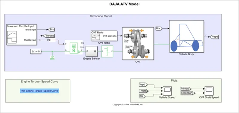
This submission contains a set of models created with Simulink, Simscape, and Simscape Driveline.

More specifically, the file contained includes explanation for : BAJA ATV model with Continuously Variable Transmission(CVT).

These models show how to build an ATV with CVT which is mostly used in BAJA competitions. Simscape and Simscape Driveline have been used to complete the system. The engine data used in the model is provided as an image which shows the Engine Speed (RPM) Vs Torque curve.

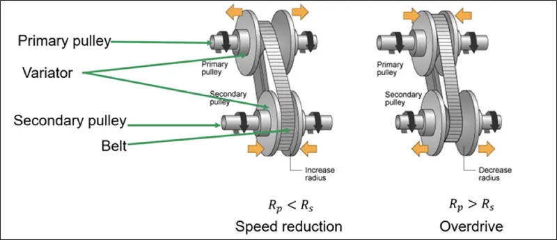
CVTs differ from traditional automatic transmissions in that they don't have gears that provide "steps" between low- and high-speed operation. Instead, the majority of them work via a pair of variable-diameter, cone-shaped pulleys connected by a steel or composite belt.

Model 1: CVT Simscpae Model

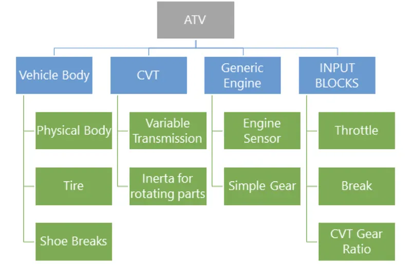
Components present:

Input System:

Here the inputs are given using Signal builder. Here we are using two signals, one for the Brake Input and another for the Throttle input. We can observe that currently there is no break input provided to the system and a constant throttle is provided which changes after 20 seconds into the simulation.

Generic Engine

• The Generic Engine block represents a general internal combustion engine. Engine types include spark-ignition and diesel. Speed-power and speed-torque parameterizations are provided.
• A throttle physical signal input specifies the normalized engine torque.
• Optional dynamic parameters include crankshaft inertia and response time lag.
• A physical signal port outputs engine fuel consumption rate based on choice of fuel consumption model. Optional speed and redline controllers prevent engine stall and enable cruise control.
• Connections F and B are mechanical rotational conserving ports associated with the engine crankshaft and engine block, respectively. Connections P and FC are physical signal output ports through which engine power and fuel consumption rate are reported.

Engine Settings:

• For this particular model we have specified the initial inertia of 1kg*m^2, & Initial velocity of 2100 rpm.
• We have used a limit of 100 rpm as speed threshold.
• We are not using any fuel consumption model or speed control model.

Engine Sensor

• The block represents an ideal mechanical rotational motion sensor, that is, a device that converts an across variable measured between two mechanical rotational nodes into a control signal proportional to angular velocity or angle. The sensor is ideal since it does not account for inertia, friction, delays, energy consumption, and so on.
• Connections R and C are mechanical rotational conserving ports and connections W and A are physical signal output ports for velocity and angular displacement, respectively

Here we observe that the rpm drops from 2100 rpm to a significant portion and then gradually picks up and rises and after 40 seconds into the motion it becomes constant.

IV Simple Gear

This simple gear is used in the simulation because we want to have a power transmission from the engine to the driver pulley for speed reduction. This has nothing to do with the CVT.

The Simple Gear block represents a gearbox that constrains the connected driveline axes of the base gear, B, and the follower gear, F, to co rotate with a fixed ratio that you specify.

Settings used:

Follower (F) to base (B) teeth ratio (NF/NB): 4

Output Shaft Rotates in the same direction as the input shaft

No Meshing losses and no Viscous losses are provided.

As we can see that the simulation would stop if we choose a higher gear ratio and would not be able to produce enough torque if we use lower values of the gear ratios we arrive for the value of 4 for which we can see that our velocity reaches a constant value after a specific point of time.

V.CVT (Continuously Variable Transmission)

• Here the two inertia blocks represent the primary pulley and the Out put shaft inertia represents the secondary pulley inertia.
• Then the Variable gear ratio block is used to model continuously variable transmission.
• Represents a variable ratio gearbox such as implemented by mechanical belt CVT, electric, or hydraulic transmissions. The physical signal input r defines the ratio of input to output angular shaft velocities
• Connections B (base) and F (follower) are mechanical rotational conserving ports. Specify the relation between base and follower rotation directions with the Output shaft rotates parameter

Input for the CVT (Continuously Variable Transmission)

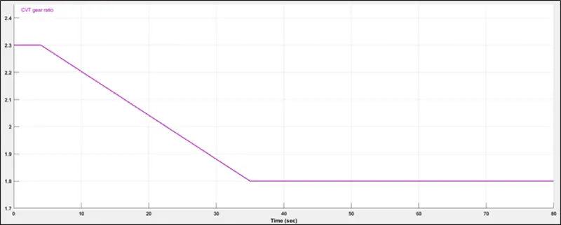
Here we can observe that a random input of the CVT gear ratio is given to the variable gear ratio block from port 1 using the CR import block.

V. Vehicle Body

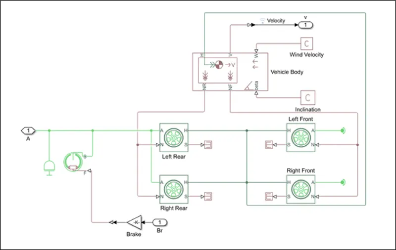
• Here we are modelling the ATV’s main frame and the wheels.

Tire (Magic Formula)

• Wheels work on the magic formula

N- Normal Force S- Slip A- Axle H-Hub

1. The Tire (Magic Formula) block models a tire with longitudinal behavior given by the Magic Formula, an empirical equation based on four fitting coefficients. The block can model tire dynamics under constant or variable pavement conditions.
2. The Tire (Magic Formula) block models the tire as a rigid wheel-tire combination in contact with the road and subject to slip.
3. When torque is applied to the wheel axle, the tire pushes on the ground (while subject to contact friction) and transfers the resulting reaction as a force back on the wheel. This action pushes the wheel forward or backward.

Assumptions and Limitations

• The Tire (Magic Formula)block assumes longitudinal motion only and includes no camber, turning, or lateral motion.
• Tire compliance implies a time lag in the tire response to the forces on it. Time lag simulation increases model fidelity but reduces simulation performance.

Double Shoe Break

• There are four wheels in which the rear wheels are connected to the output shaft from the CVT through the axles making it a rear wheel drive.
• A double shoe breaks is also connected to the rear wheel axels which is used to apply break power to the rear wheels.

Vehicle Body

• Here the body is connected to the wheels and the hub of the wheels according to the connections to simulate the working of the body.
• Here we can provide the mass of the vehicle and carry out different simulations for the torque and velocity depending on the mass provided.
• Β represents the angle of inclination of the road at which the vehicle is travelling.
• There is a port ‘W’ which is used to provide head wind speed that the car will face.

Settings for the Vehicle Body:

OUTPUT

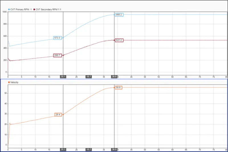
We can observe that the secondary pulley is rotating at a lower rpm than the primary pulley and hence we can see that this arrangement is to supply Torque to the engine.

Now if we change the CVT gear ratio input and reduce it to a value less than 1 we can observe the effect on the RPM of the secondary pulley and then we further increase the CVT gear ratio and we can observe the transition into the rpm as well the velocity of the vehicle.

We can observe that after we start increasing the CVT gear ratio, the secondary rpm starts to drop and so doe the velocity of the vehicle.

BAJA ATV DASHBOARD MODEL

This model is same as the CVT model, but here the input is given through the dashboard control knobs. So, the Throttle input knob and the brake input knob is connected to the constant block which provides the input while the model is running for infinite time. This helps us to create various scenarios while the simulation is running.

OUTPUT

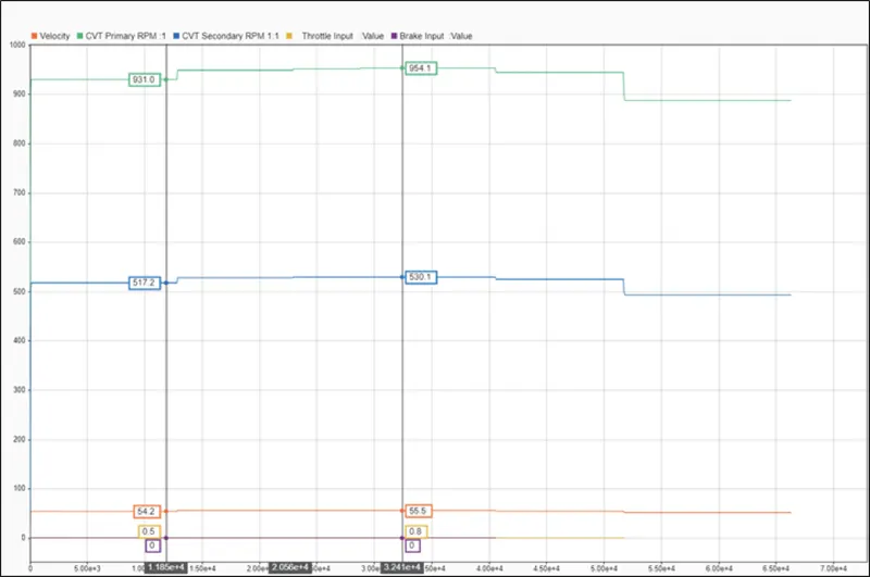
We can observe the effect of change of the throttle on the vehicle speed.

CVT Mapped Model

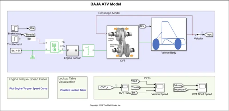
Here we can observe that the CVT gear ratio is not given through the signal builder rather here we are using look up table as shown below.

%% Load and simulate the model

cvtModel_data

sim('cvtModel_data')

%% Visualize the lookup table

plot(vehicle_speed,cvt_ratio,'r','LineWidth',2)

xlabel ('Vehicle Speed (km/hr)')

ylabel ('CVT Ratio')

title ('Lookup Table Visualization')

This is a visualization of Look up table, here Vehicle speed is working as the input vector or x. And we are obtaining the CVT based on the relation described by the user to evaluate the CVT.

The PS Lookup Table (1D) block computes an approximation to some function f=f(x) given data vectors x and f. Both the input and the output are physical signals.

You define the lookup table by specifying the Table grid vector parameter as a 1-by-n vector (x data vector) and the Table values parameter as a 1-by-n vector (f data vector). The block generates output based on the input values using the selected interpolation and extrapolation methods.

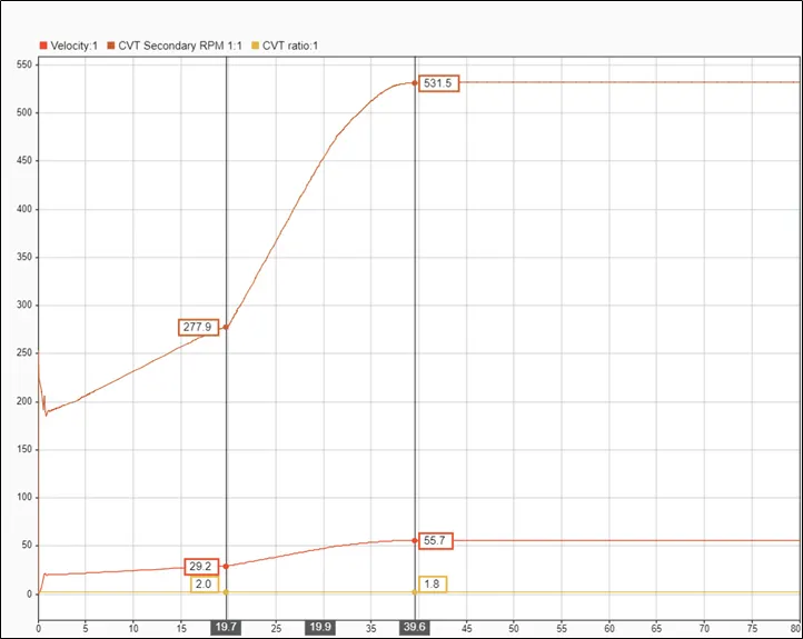
In this way we can model a continuously varying transmission based on the vehicle speed as this is taking feed back from the vehicle speed and then calculating its CVT.

OUTPUT

CONCLUSION:

Simulation of a BAJA ATV using CVT is simulated in two ways to visualize the effect of CVT on Vehicle velocity and secondary rpm. Based on this we can simulate multiple situations and designs for different models for ATV designs using the specks of that particular model.