Project

AIM:- Carry out a system-level simulation of an all-terrain vehicle.

Prepare a technical report explaining the model properties & comments on the results.

THEORY:- An all-terrain vehicle (ATV), also known as a quad, as defined by the American National Standards Institute (ANSI) is a vehicle that travels on low-pressure tires, with a seat that is straddled by the operator, along with handlebars for steering control. As the name implies, it is designed to handle a wider variety of terrain than most other vehicles. Although it is a street-legal vehicle in some countries, it is not street-legal within most states, territories, and provinces of Australia.

By the current ANSI definition, ATVs are intended for use by a single operator, although some companies have developed ATVs intended for use by the operator and one passenger. These ATVs are referred to as tandem ATVs

The rider sits on and operates these vehicles like a motorcycle, but the extra wheels give more stability at slower speeds. Although most are equipped with three or four wheels, six-wheel models exist for specialized applications. Multiple-user analogues with side-by-side seating are called Utility Terrain vehicle (UTV) to distinguish the classes of vehicle. Both classes tend to have similar powertrain parts.

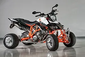
CASE STUDY 1:- Analysis of CVT Baja model

About CVT

CONTINUOUSLY VARIABLE TRANSMISSION:- A continuously variable transmission (CVT) is an automatic transmissions that can change seamlessly through a continuous range of gear ratios. This contrasts with other transmissions that provide a limited number of gear ratios in fixed steps. The flexibility of a CVT with suitable control may allow the engine to operate at a constant RPM while the vehicle moves at varying speeds.

CVTs are used in automobiles, tractors, motor scooters, snowmobiles and earthmoving equipment.

The most common type of CVT uses two pulleys connected by a belt or chain, however several other designs have also been used at times.

Here we will use a pulley based CVT

The image below is of a pulley based CVT

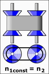
The pulleys will be conical shaped and a belt is passed over these pulleys. The reason being conical shaped is that we can alter the diameter of the two pulleys thereby varying the gear ratios. The diameter of the pulleys can be increased or decreased by moving the two conical parts of the pulleys in and out. When the diameter of the primary pulley is increased and the diameter of the secondary pulley is decreased we will see an increase in ‘Output speed’ and when the reverse condition is applied the ‘Output speed’ is decreased. Hence we can attain a number of ‘Gear ratios’.

In the given model of ‘ATV’ we will provide a signal for ‘Brake’ and ‘Throttle’ through a ‘Signal builder block’. The ‘Throttle’ signal will go directly into the ‘Generic Engine block’.

About the ‘Generic Engine Block’.

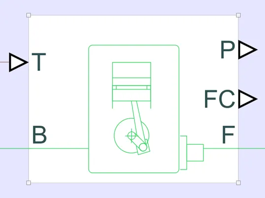
It consists of five ports.

The ‘T’ port is the Physical signal input port specifying the normalized engine throttle level.

The ‘B’ port is the Rotational conserving port representing the engine block, which will be connected to the mechanical reference block.

The ‘F’ port is the Rotational Conserving port representing the engine crankshaft, which will be connected to the input of the ‘Engine Sensor Block’.

The ‘P’ and the ‘FC’ block will not be connected as of we don’t need it now, since it signifies the ‘instantaneous engine power’ and the ‘Fuel consumption rate’ respectively. The ‘FC’ in the ‘Generic Engine Block’ should be set to ‘No Fuel Consumption’ to increase the simulation speed. If you select any other option for the Fuel consumption model, the block solves a nonlinear equation that is required for calculating fuel consumption. The block solves the equation even if the FC port, which reports the fuel consumption rate, is not connected to another block. When the parameter is set to No fuel consumption, the block does not calculate fuel consumption, even if the FC port is connected to another block.

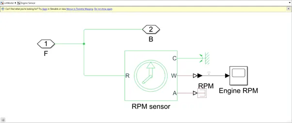
ENGINE SENSOR BLOCK

The output from the ‘Generic Engine Block’ will be the input to the ‘Engine sensor block’ The below diagram is of the ‘Engine Sensor Block’.

SIGNAL BUILDER FOR THROTTLE AND BRAKE

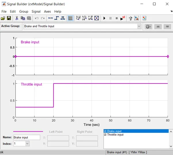
Here we will give these two signals through the ‘Signal Builder Block’ i.e the ‘Brake Input’ and the ‘Throttle Input’.

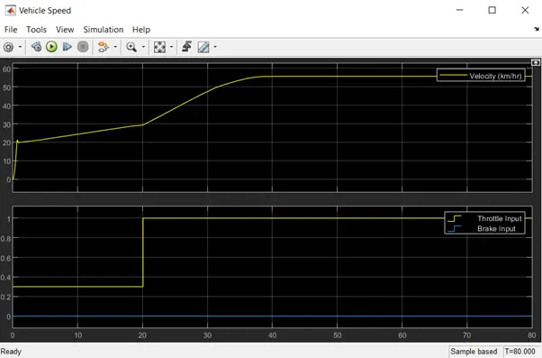
The ‘Brake Input’ will be given as ‘0’ and the ‘Throttle Input’ will be given as ‘0.3’ for the first 20 seconds and for the rest of the time will be given as ‘1’.

Now we will observe the Scope Block attached to the RPM sensor.

The output of the ‘Engine Sensor Block’ will be connected to the Input of ‘Simple Gear’ block where we will assign the gear ratio as ‘4’.

Then the output of the ‘Simple gear block’ will be connected to the block representing the ‘CVT’.

The below image is of the ‘CVT’ block

CVT BLOCK

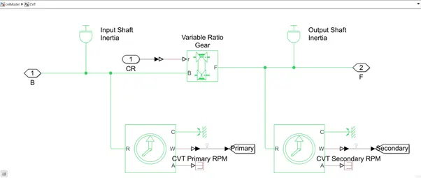
Here the Input shaft will receive the speed of the output of the ‘Simple Gear Block’. A ‘Signal Builder Block’ will be used to provide different gear ratios and will be connected to the ‘Variable Ratio Gear’ block. After taking these two Inputs the speed of the Output shaft will be calculated. There will be Two sensors attached to the ‘Primary Shaft’ and the ‘Secondary Shaft’ to observe the Input and Output speeds under the ‘Scope Block’.

SIGNAL BUILDER BLOCK FOR CVT:-

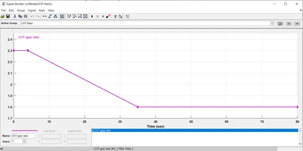
Here we will provide a CVT gear ratio to the ‘Variable Gear Ratio’ block present in the ‘CVT’ block which will take two inputs i.e from ‘Signal builder’ block and ‘Simple gear’ block and will calculate the speed of the Output shaft based on the CVT ratio provided by the ‘Signal Builder’ block.

VEHICLE BODY BLOCK

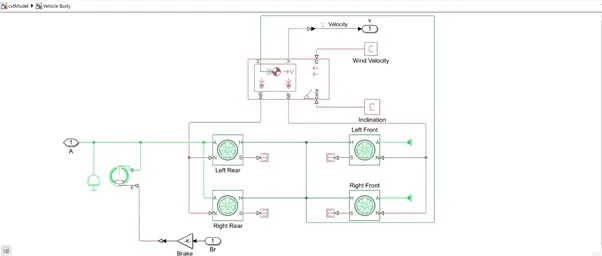
The Vehicle Body block represents a two-axle vehicle body in longitudinal motion. The vehicle can have the same or a different number of wheels on each axle. For example, two wheels on the front axle and one wheel on the rear axle. The vehicle wheels are assumed identical in size. The vehicle can also have a center of gravity (CG) that is at or below the plane of travel.

The block accounts for body mass, aerodynamic drag, road incline, and weight distribution between axles due to acceleration and road profile. Optionally include pitch and suspension dynamics. The vehicle does not move vertically relative to the ground.

The block has an option to include an externally-defined mass and an externally-defined inertia. The mass, inertia, and center of gravity of the vehicle body can vary over the course of simulation in response to system changes.

Model

The vehicle axles are parallel and form a plane. The longitudinal, x, direction lies in this plane and perpendicular to the axles. If the vehicle is traveling on an incline slope, β, the normal, z, direction is not parallel to gravity but is always perpendicular to the axle-longitudinal plane.

The below image is of the ‘Vehicle Body’

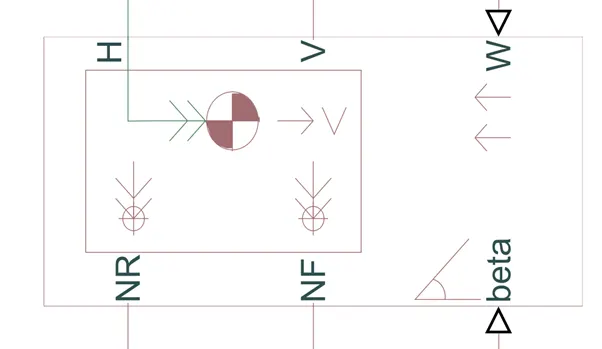
PORTS:-

Input Ports

W — Headwind speed, m/s

Physical signal input port for headwind speed.

beta — Road incline angle, rad
Physical signal input port for road incline angle.

CG — Center of gravity, m
Physical signal input port for the center of gravity, in m, of the externally-defined mass relative to the CG of the vehicle body.

M — Mass, kg
Physical signal input port for the mass, in kg, of the externally-defined mass.

J — External moment of inertia, kg*m^2
Physical signal input port for the moment of inertia, in kg*m^2, of the externally-defined mass.

Output ports

V — Longitudinal velocity, m/s
Physical signal output port for vehicle longitudinal velocity.

NF — Front axle normal force, N
Physical signal output port for normal force on the front axle. Wheel forces are considered positive if acting downwards.

NR — Rear axle normal force, N
Physical signal output port for normal force on the rear axle. Wheel forces are considered positive if acting downwards.

H — Horizontal motion
mechanical translational

Conserving port associated with the horizontal motion of the vehicle body. Connect tire traction motion to this port.

TIRES

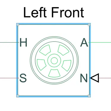
The Tire (Magic Formula) block models a tire with longitudinal behavior given by the Magic Formula, an empirical equation based on four fitting coefficients. The block can model tire dynamics under constant or variable pavement conditions.

The longitudinal direction of the tire is the same as its direction of motion as it rolls on pavement. This block is a structural component based on the Tire-Road Interaction (Magic Formula) block.

To increase the fidelity of the tire model, you can specify properties such as tire compliance, inertia, and rolling resistance. However, these properties increase the complexity of the tire model and can slow down simulation. Consider ignoring tire compliance and inertia if simulating the model in real time or if preparing the model for hardware-in-the-loop (HIL) simulation.

Tire Model

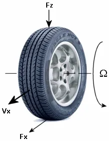
The Tire (Magic Formula) block models the tire as a rigid wheel-tire combination in contact with the road and subject to slip. When torque is applied to the wheel axle, the tire pushes on the ground (while subject to contact friction) and transfers the resulting reaction as a force back on the wheel. This action pushes the wheel forward or backward. If you include the optional tire compliance, the tire also flexibly deforms under load.

The figure shows the forces acting on the tire. The table defines the tire model variables.

PORTS:-

Input Ports

N — Normal force
physical signal

Physical signal input port associated with the normal force acting on the tire. The normal force is positive if it acts downward on the tire, pressing it against the pavement.

Output ports

S — Slip
physical signal

Physical signal output port associated with the relative slip between the tire and road.

A — Axle
mechanical rotational

Mechanical rotational port associated with the axle that the tire sits on.

H — Hub
mechanical translational

Mechanical translational port associated with the wheel hub that transmits the thrust generated by the tire to the remainder of the vehicle.

BRAKE

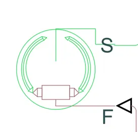
The Double-Shoe Brake block represents a frictional brake with two pivoted rigid shoes that press against a rotating drum to produce a braking action. The rigid shoes sit inside or outside the rotating drum in a diametrically opposed configuration. A positive actuating force causes the rigid shoes to press against the rotating drum. Viscous and contact friction between the drum and the rigid shoe surfaces cause the rotating drum to decelerate.

Double-shoe brakes provide high braking torque with small actuator deflections in applications that include motor vehicles and some heavy machinery. The model employs a simple parameterization with readily accessible brake geometry and friction parameters.

PORTS

Input Ports

F — Actuating force
physical signal

Physical signal input port associated with the applied actuating force.

Output Ports

S — Drum shaft rotation
rotational mechanical

Rotational conserving port associated with the rotating drum shaft.

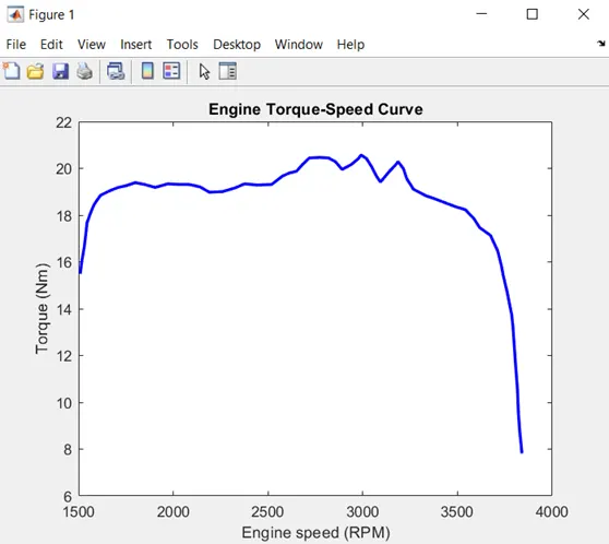
TORQUE VS SPEED CURVE

OUTPUTS:-

ENGINE RPM

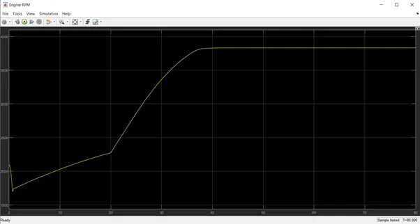
Here we can observe that as the ‘Throttle’ is increased the RPM of the engine also Increases and after sometime the Engine RPM achieves is highest speed i.e around 3850 RPM.

VEHICLE SPEED

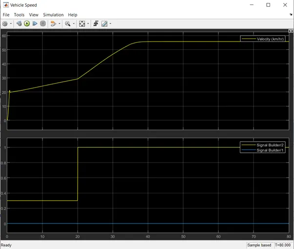
Here we can observe that when the value of the ‘Throttle’ is increased the output speed of the vehicle also increases gradually.

CVT SHAFT SPEED

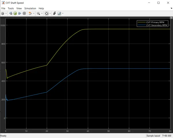
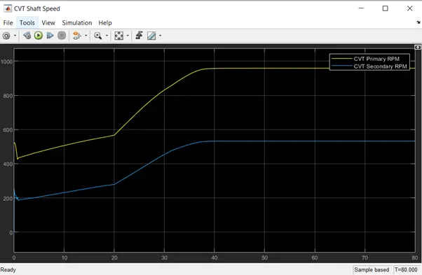
As the speed of the primary shaft increases, the speed of the secondary shaft also increases. After sometime both the speeds attains a constant maximum value.

The reason being the Speed of the primary shaft greater than the Speed of the Secondary shaft is because of the CVT ratios provided and the ‘Torque’ required to start and move the vehicle. Since the Secondary shaft has low speed at the start, it will provide sufficient ‘Torque’ to start the vehicle.

Case study 2:- Analysis of CVT Baja model using a Dashboard

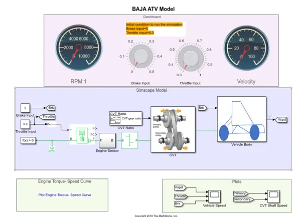
Everything will be same as the previous case, instead in this one we will use a Dashboard for controlling the ‘Throttle’ and ‘Brake’ values.

There are two knobs for ‘Throttle’ and ‘Brake’ that we can manipulate while the simulation is going on and observe how the vehicle is performing.

The below is the image of the model

OUTPUTS:-

Engine RPM

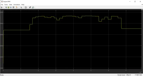
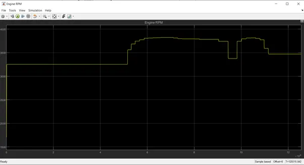
The above image represents the Engine RPM when the ‘Throttle’ values are changed. The increase in the throttle values provides more Engine RPM.

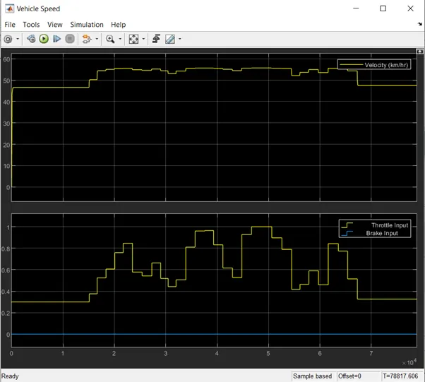
Vehicle speed

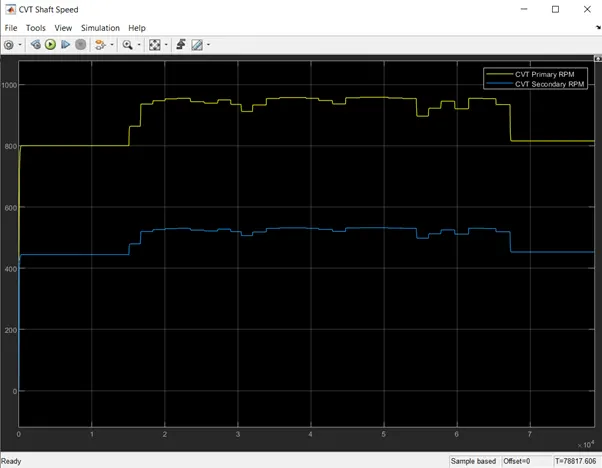
CVT Shaft speed

Case study 3:- Analysis of CVT Baja model using Lookup table

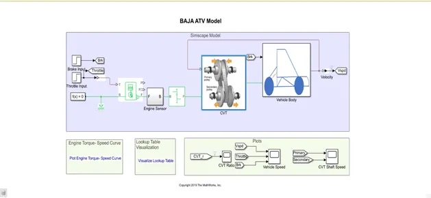
Image of the model using Lookup table is shown below

Lookup Table

A lookup table is an array of data that maps input values to output values. You can use a lookup table to model your system, and tune the table data using measured data from your system. The resulting tablerepresents a static system.

The behavior of actual physical systems often varies with time due to wear, environmental conditions, and manufacturing tolerances. Use adaptive lookup tables to model the time-varying behavior of physical plants. Adaptive lookup table values update dynamically with incoming input-output data as the model is simulated.

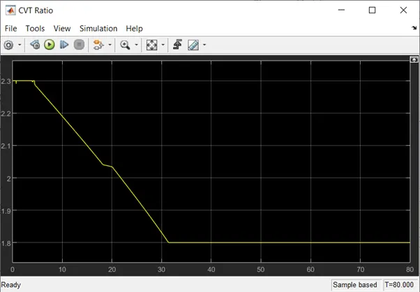
In the above model without using a closed loop we are providing some random values of the CVT ratio and checking the performance of the vehicles.

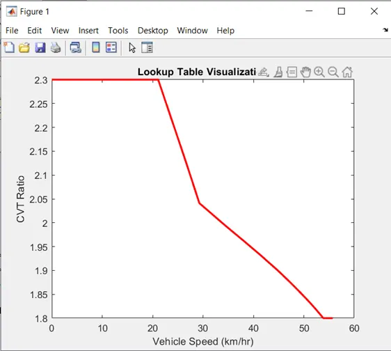
In practical case the CVT ratio will depend on the vehicle velocity. That is why we will simulate a closed loop model which is built using the lookup table.

We have written a script which is shown below which will give a relation between the CVT ratio & vehicle speed.

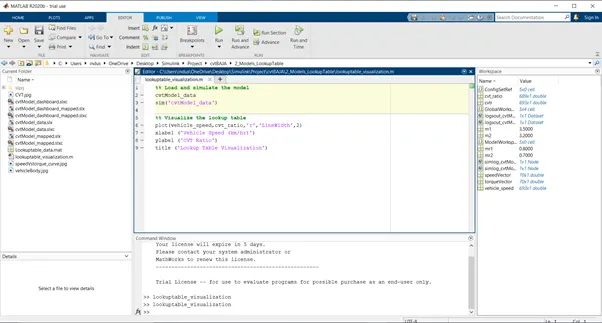
In the above model the velocity value which is coming out of the vehicle body block is taken as the input to the CVT block and is given to the lookup table block in the CVT block as shown below.

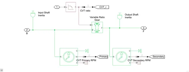
According to the velocity of the vehicle the lookup table will calculate the new CVT ratio and provide it to the ‘Variable gear ratio’ block and we will get different outputs as shown below.

OUTPUTS:-

Below will be the observations. We see that an increase in the throttle values results in an increase in the output speed.

CVT Ratio

VECHICLE SPEED

CVT SHAFT SPEED

CASE STUDY 4:- Analysis of CVT BAJA ATV using lookup table and dashboard

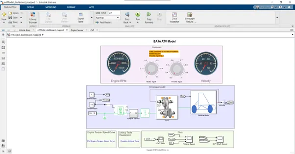
Everything will reamain same as the above ‘CASE STUDY 3’, exept a Dashboard will be introduced where it will contain a switch for ‘Throttle’ and ‘Brake’.

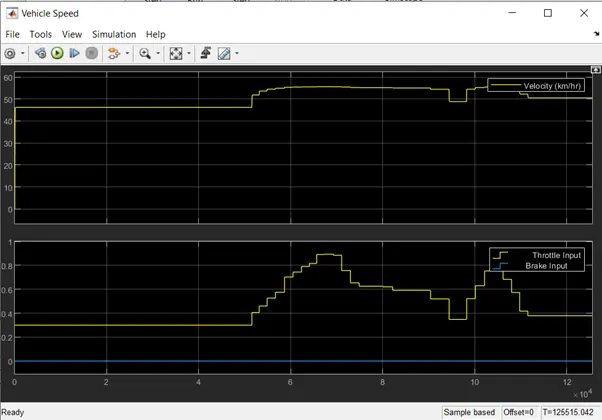
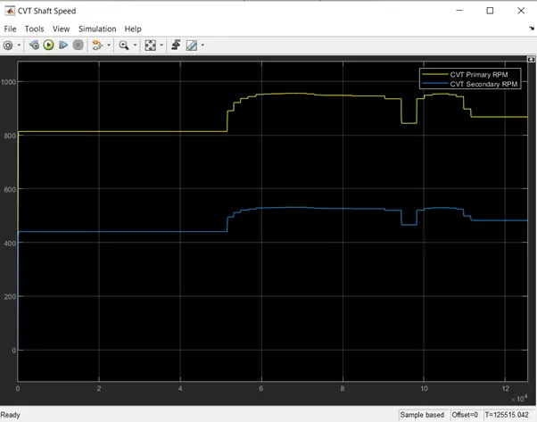
From the Dashboard we can run the simulation and during simulation time we can change the ‘Throttle’ value and ‘Brake’ value and can observe how the ATV will be performing.

The model is given below

OUTPUTS:-

Engine RPM

Vehicle Speed

CVT Shaft speed

CONCLUSION:- The above four cases has been observed for CVT Baja ATV model