Project 1 - Parsing NASA thermodynamic data

OBJECTIVE

The objective of this project is to calculate the thermodynamic properties (specific heat, entropy and enthalpy) for various species using NASA Thermodynamic data, calculate their molecular weight and plot thermodynamic properties with the temperature.

STEPS TAKEN

Main program

Parsing NASA thermodynamic data

• THERMO.dat file is opened using fopen, and the contents are read using fgetl.
• Global and local temperature ranges are extracted from the files.

Reading coefficients

• For each species high temperature and low temperature coefficients are extracted.

Calculating thermodynamic properties

• Depending on the temperature, either the high temperature or low temperature coefficients are used.
• The formulas provided are used to calculate Cp, H and S.

Molecular weight calculation

• A sub function is used to calculate molecular weight based on the species composition.

Plotting and saving result

• For each species three plots (Cp vs T, H vs T, S vs T) are generated.
• The plots are saved as .jpg files in a folder named after the species. Then fclose is used to close the file THERMO.dat.

Code

clear all

close all

clc

% Parsing NASA thermodynamic data

% Reading data file

f1 = fopen('THERMO.dat','r');

line1 = fgetl(f1);

line2 = fgetl(f1);

header = strsplit(line2,' ');

R = 8.314; % Universal gas constant

% Global temperature

global_low_temp = str2double(header{2});

global_mid_temp = str2double(header{3});

global_high_temp = str2double(header{4});

% Skipping unwanted lines

for i = 1:3

fgetl(f1);

end

% Reading species data

for j = 1:53

line_1 = fgetl(f1);

line = strsplit(line_1,' ');

species = line{1};

a = flip(line);

% Local temperature

local_low_temp = str2double(a{4});

local_mid_temp = str2double(a{2});

local_high_temp = str2double(a{3});

% Temperature range

temp = linspace(local_low_temp,local_high_temp,1000);

% Storing values of line

line_2 = fgetl(f1);

x = strfind(line_2,'E');

line_3 = fgetl(f1);

y = strfind(line_3,'E');

line_4 = fgetl(f1);

z = strfind(line_4,'E');

% Higher temperature coefficient

a1 = str2double(line_2(1:x(1)+3));

a2 = str2double(line_2(x(1)+4:x(2)+3));

a3 = str2double(line_2(x(2)+4:x(3)+3));

a4 = str2double(line_2(x(3)+4:x(4)+3));

a5 = str2double(line_2(x(4)+4:x(5)+3));

a6 = str2double(line_3(1:y(1)+3));

a7 = str2double(line_3(y(1)+4:y(2)+3));

% Lower temperature coefficient

b1 = str2double(line_3(y(2)+4:y(3)+3));

b2 = str2double(line_3(y(3)+4:y(4)+3));

b3 = str2double(line_3(y(4)+4:y(5)+3));

b4 = str2double(line_4(1:z(1)+3));

b5 = str2double(line_4(z(1)+4:z(2)+3));

b6 = str2double(line_4(z(2)+4:z(3)+3));

b7 = str2double(line_4(z(3)+4:z(4)+3));

% Calculating Specific heat , Enthalpy and Entropy

if temp <= local_mid_temp

Cp = R.*(b1+(b2.*temp)+(b3.*(temp.^2))+(b4.*(temp.^3))+(b5.*(temp.^4)));

H = R*temp.*(b1+(b2.*(temp./2))+(b3.*((temp.^2)./3))+(b4.*((temp.^3)./4))+(b5.*((temp.^4)./5))+(b6./temp));

S = R.*((b1.*log(temp))+(b2.*temp)+(b3.*((temp.^2)./2))+(b4.*((temp.^3)./3))+(b5.*((temp.^4)./4))+b7);

else

Cp = R.*(a1+(a2.*temp)+(a3.*(temp.^2))+(a4.*(temp.^3))+(a5.*(temp.^4)));

H = R*temp.*(a1+(a2.*(temp./2))+(a3.*((temp.^2)./3))+(a4.*((temp.^3)./4))+(a5.*((temp.^4)./5))+(a6./temp));

S = R.*((a1.*log(temp))+(a2.*temp)+(a3.*((temp.^2)./2))+(a4.*((temp.^3)./3))+(a5.*((temp.^4)./4))+a7);

end

% Calculating molecular weight

W = Molecular_weight(species);

% Creating folder for species data

current_directory = pwd;

mkdir(species);

cd(species);

% Plotting data

% Specific heat (Cp) VS Temperature(T)

figure(1)

plot(temp,Cp,'LineWidth',3,'Color','b')

xlabel('Temperature (k)')

ylabel('Specific heat (kj/kg k)')

title(sprintf('Specific heat VS Temperature of %s',species))

saveas(figure(1),'Specific heat.jpg')

grid on

% Enthalpy (H) VS Temperature(T)

figure(2)

plot(temp,H,'LineWidth',3,'Color','r')

xlabel('Temperature (k)')

ylabel('Enthalpy (kj/kg)')

title(sprintf('Enthalpy VS Temperature of %s',species))

saveas(figure(2),'Enthalpy .jpg')

grid on

% Entropy (S) VS Temperature(T)

figure(3)

plot(temp,S,'LineWidth',3,'Color','g')

xlabel('Temperature (k)')

ylabel('Entropy (kj/k)')

title(sprintf('Entropy VS Temperature of %s',species))

saveas(figure(3),'Entropy.jpg')

grid on

cd(current_directory)

end

fclose(f1);

Sub program

• Defines a list of elements and their respective atomic number
• A variable W (molecular weight) is set to 0.
• The program looks at each letter in the species name. if it matches an element in the reference table, its atomic weight is added to W.
• If there’s a number after an element, the program multiplies the atomic weight of that element by the number and add it to W.
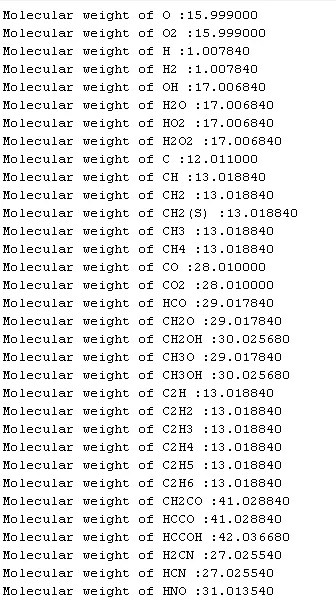
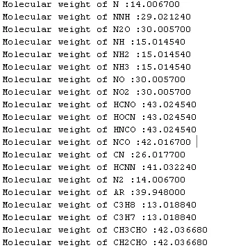
• The calculated molecular weight is printed in the command window.

Code

function[W] = Molecular_weight(species)

elements = ['H','C','N','O','Ar'];

atomic_weight = [1.00784 12.011 14.0067 15.999 39.948];

W = 0;

for i = 1:length(species)

for j = 1:length(elements)

if strcmp(species(i),elements(j))

W = W + atomic_weight(j);

end

end

n = str2num(species);

if n > 1

W = W + (atomic_weight(j).*(n-1));

end

end

% Print results

fprintf('Molecular weight of %s :',species);

fprintf('%f',W);

disp(' ');

end

RESULTS

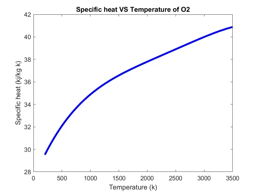
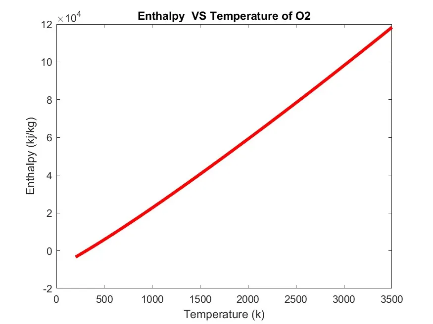
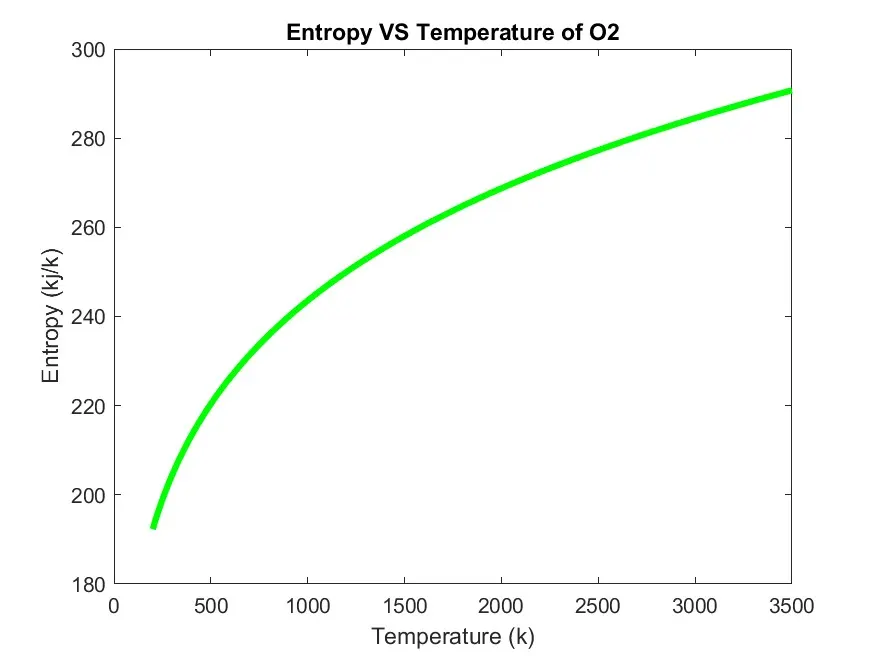
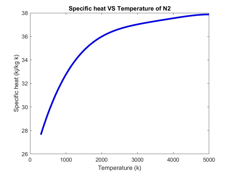
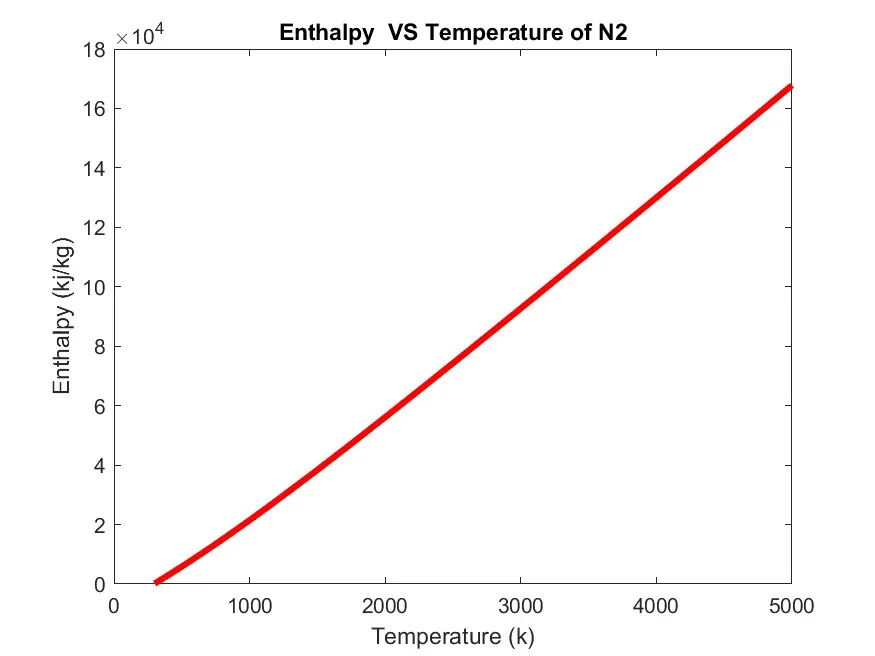
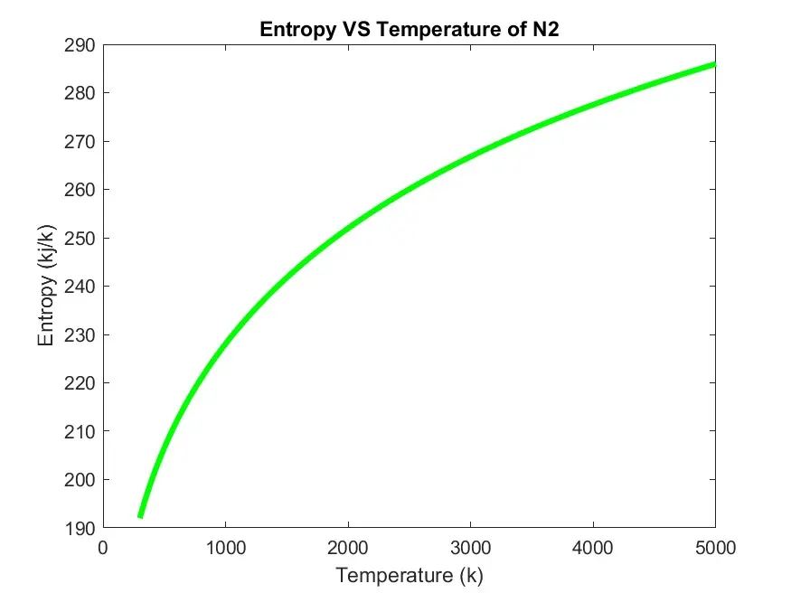
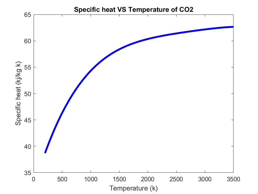
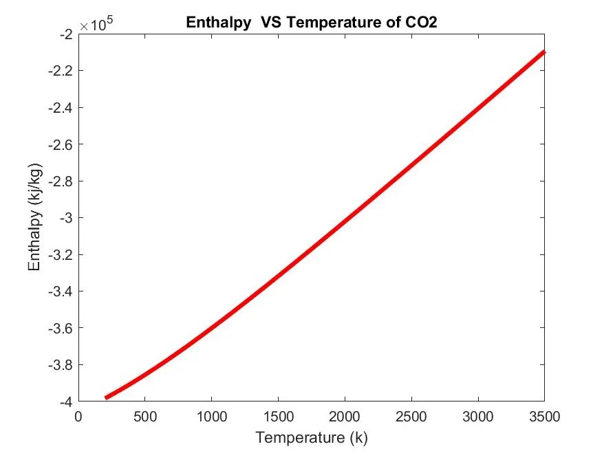
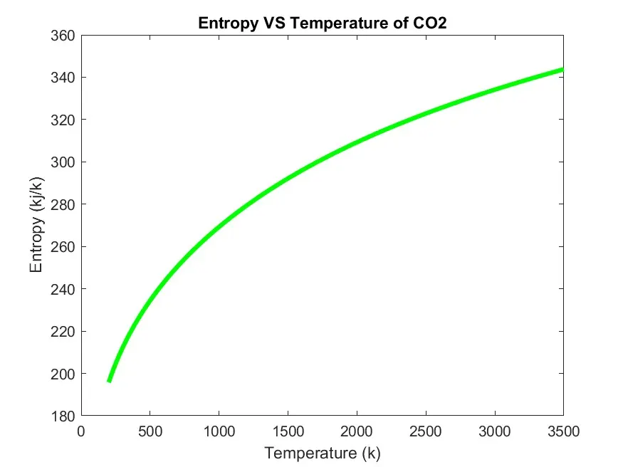
The program generates and saves the plots for Cp, H and S against temperature for all species. Below are example for O2, N2 and CO2.

O2

Specific heat vs Temperature

Enthalpy vs Temperature

Entropy vs Temperature

N2

Specific heat vs Temperature

Enthalpy vs Temperature

Entropy vs Temperature

CO2

Specific heat vs Temperature

Enthalpy vs Temperature

Entropy vs Temperature

Molecular weights for each species are calculated and displayed in the command bar.

Screenshots showing folders created for each species containing respective plots.