Project 1 - Parsing NASA thermodynamic data

Aim:- To write a program in MATLAB to parse NASA thermodynamics data file.

Objective:-

• Write a function that extracts the 14 coefficients and calculates the enthalpy,entropy and specific heats for all the species in the data file.
• Calculating molecular weight of each species.
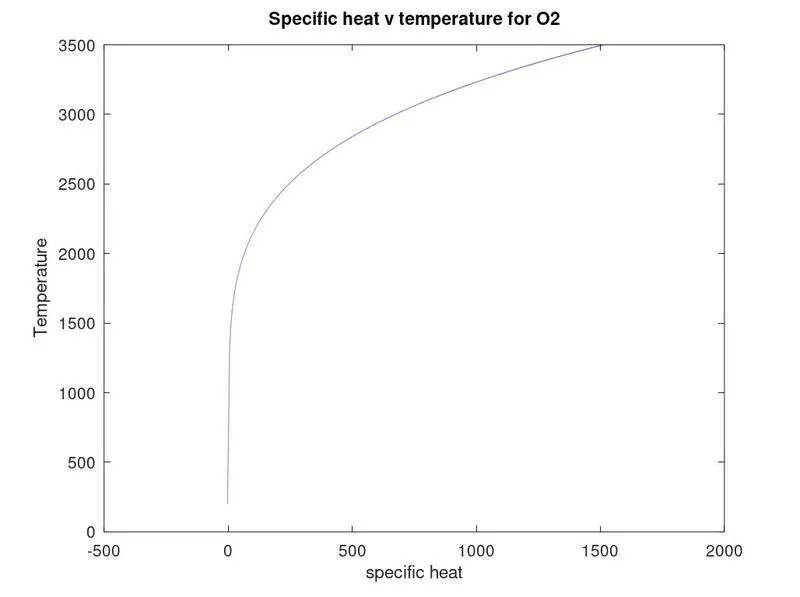
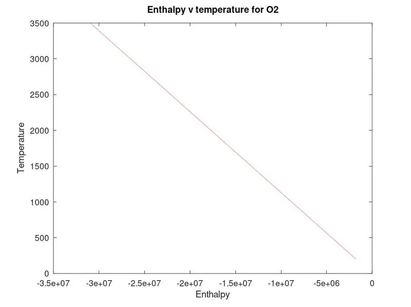
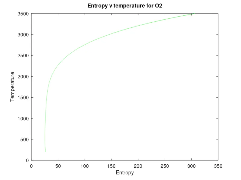
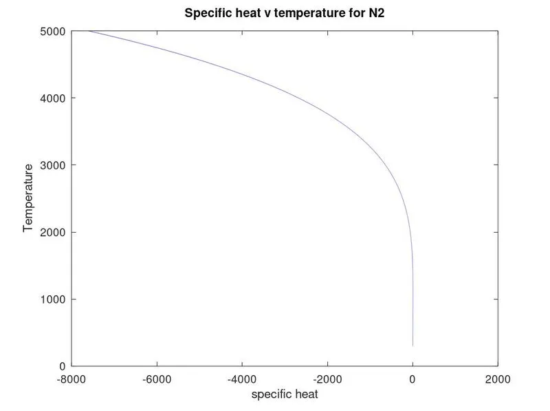
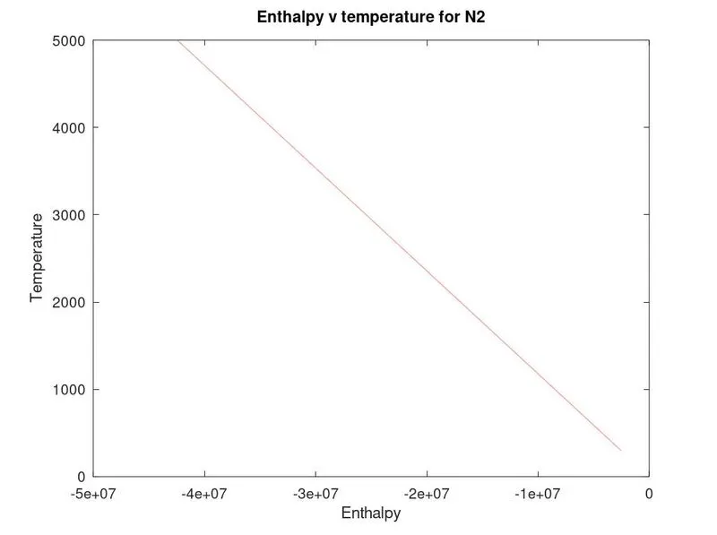
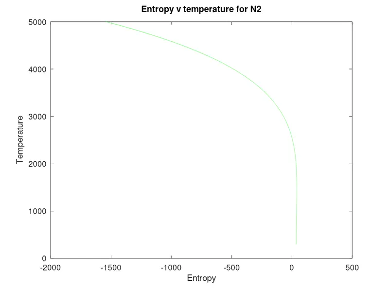
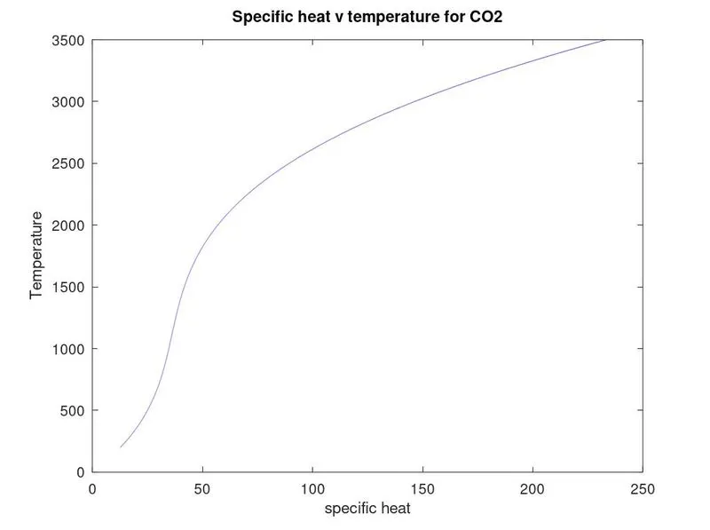
• Plotting the specific heat,enthalpy and entropy for the local temperature range.
• Saving the plots as images with appropriate names and dumping them in seperate folders for each species.

Mathematical equation:-

Specific heat equation:

`Cp = R*(a1 + (a2*T) + (a3*(T.^2))````4*(T.^3)``+ (a5*(T.^4)))`

Enthalphy equation:

`H``= R*(a1 + (a2*T/2) + (a3*(T.^2)/3) + (a4*(T.^3)/4) + (a5*(T.^4)/5) + (a6*(T)))`

Entropy equation:

`S = R*((a1*log(T)) + (a2*T) + (a3*(T.^2)/2) + (a4*(T.^3)/3) + (a5*(T.^4)/4) + a7)`

Program:-

clear all
close all
clc

f1 = fopen('THERMO.dat', 'r');
tline = fgetl(f1);

%Universal gas constant(J/K mol)
R = 8.314;

%Loop to run the first 4 lines of the data file
for i = 1:4
    
    fgetl(f1);
    
end

%Loop to obtain data and get the plots for each species

for i = 1:53
    
    %Obtaining the name of the species and converting to a string value for convenience
    
    tline1 = fgetl(f1);
    a = strsplit(tline1, ' ');
    species_cell = a(1);
    species = char(species_cell);
    
    %Finding the local values of temperature for each species

    str1 = strfind(tline1, '.');
    low_temp_range = str2num(tline1(str1(1)-4:str1(1)+3));
    high_temp_range = str2num(tline1(str1(2)-4:str1(2)+3));
    med_temp_range = str2num(tline1(str1(3)-4:str1(3)+3));
    
    %Obtaining the coefficients from the subsequent three lines
    
    tline2 = fgetl(f1);
    str = strfind(tline2, 'E');
    a1 = str2num(tline2(1:str(1)+3));
    a2 = str2num(tline2(str(1)+4:str(2)+3));
    a3 = str2num(tline2(str(2)+4:str(3)+3));
    a4 = str2num(tline2(str(3)+4:str(4)+3));
    a5 = str2num(tline2(str(4)+4:str(5)+3));
    
    tline3 = fgetl(f1);
    a6 = str2num(tline3(1:str(1)+3));
    a7 = str2num(tline3(str(1)+4:str(2)+3));
    a8 = str2num(tline2(str(2)+4:str(3)+3));
    a9 = str2num(tline3(str(3)+4:str(4)+3));
    a10 = str2num(tline3(str(4)+4:str(5)+3));
    
    tline4 = fgetl(f1);
    a11 = str2num(tline4(1:str(1)+3));
    a12 = str2num(tline4(str(1)+4:str(2)+3));
    a13 = str2num(tline4(str(2)+4:str(3)+3));
    a14 = str2num(tline4(str(3)+4:str(4)+3));
    
    %a1-a7 are low temperature coefficients, a8-a14 are high temperature coefficients
    
    %Calculating molecular weight of each species

    Molecular_weight = molecular_wt(species);
    sprintf('Molecular weight of %s = %d',species, Molecular_weight)
    
    %Defining T
    T = low_temp_range:high_temp_range;
    
    %Obtaining the values for Cp, enthalpy and entropy using the coefficients  
 
    if (T>med_temp_range)

        %specific heat       
        Cp = R*(a1 + (a2*T) + (a3*(T.^2)) + (a4*(T.^3)) + (a5*(T.^4)));

        %Enthaply
        H = R*(a1 + (a2*T/2) + (a3*(T.^2)/3) + (a4*(T.^3)/4) + (a5*(T.^4)/5) + (a6*(T)));

        %Entropy
        S = R*((a1*log(T)) + (a2*T) + (a3*(T.^2)/2) + (a4*(T.^3)/3) + (a5*(T.^4)/4) + a7);
        
    else 
        
        %specific heat       
        Cp = R*(a8 + (a9*T) + (a10*(T.^2)) + (a11*(T.^3)) + (a12*(T.^4)));

        %Enthaply
        H = R*(a8 + (a9*T/2) + (a10*(T.^2)/3) + (a11*(T.^3)/4) + (a12*(T.^4)/5) + (a13*(T)));

        %Entropy
        S = R*((a8*log(T)) + (a9*T) + (a10*(T.^2)/2) + (a11*(T.^3)/3) + (a12*(T.^4)/4) + a14);
        
    end
    
    %Creating the folder for the species
        t = sprintf('%s', species);
        mkdir(t);
        
        %Going in to the folder of the species to save the plots
        cd(t)   
        
        
        %Plotting the curves
        %Cp v temperature plot
        figure(1)
        plot(Cp,T, 'b');
        xlabel('specific heat')
        ylabel('Temperature')
        Cp_text = sprintf('Specific heat v temperature for %s', species);
        title(Cp_text);
        saveas(gcf, 'Cp.jpg'); 
        
        %Enthalpy v temperature plot
        figure(2)
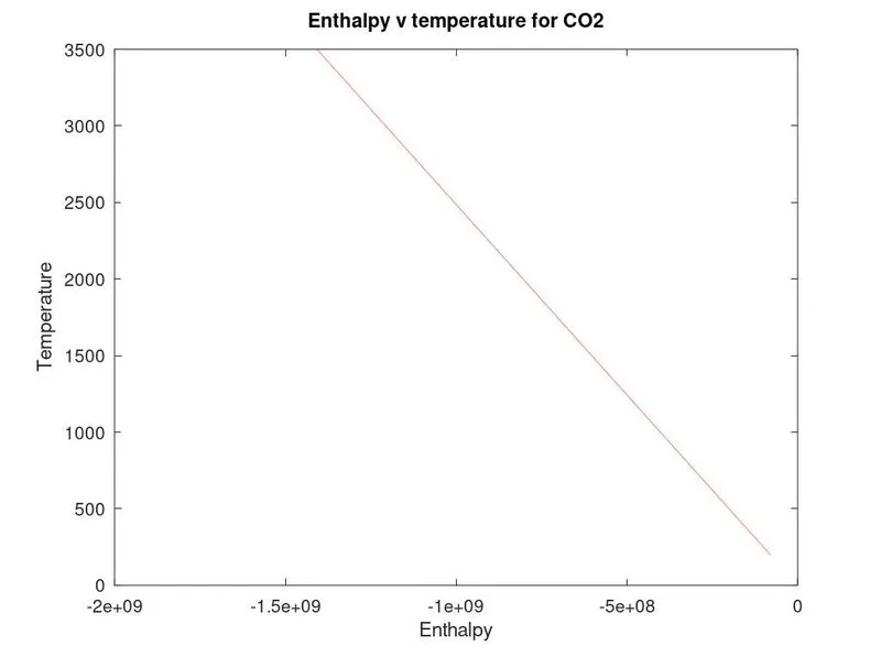
        plot(H, T, 'r');
        xlabel('Enthalpy')
        ylabel('Temperature')
        H_text = sprintf('Enthalpy v temperature for %s', species);
        title(H_text);
        saveas(gcf, 'H.jpg');
        
        %Entropy v temperature plot
        figure(3)
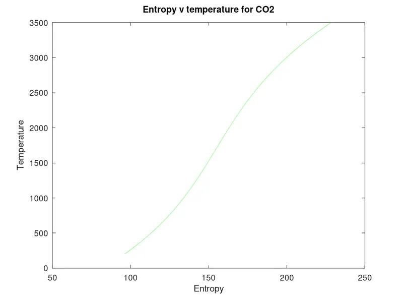
        plot(S, T, 'g');
        xlabel('Entropy')
        ylabel('Temperature')
        S_text = sprintf('Entropy v temperature for %s', species);
        title(S_text);
        saveas(gcf, 'S.png');
        
         %Going back to the previous directory
        cd ..;
end

Function to determine the molecular weights of each species:

function [out] = m_wt(spec)

%Defining the elements
elements=['H','C','N','O','R']; 

%Atomic weights of each element
Atomic_Weight = [1 12 14 16 40]; 
out=0; 

%Looping for each element inside each species and finding the atomic weight
for i=1:length(spec) 
    for j=1:length(elements) 
        if strcmp(spec(i),elements(j)) 
            out= out + Atomic_Weight(j); 
            p=j; 
        end
    end
    
    %loop to multiply the coefficients of the elements if greater than 1.
    n=str2double(spec(i)); 
    if n>1 
        out = out + (Atomic_Weight(p))*(n-1); 
    end
end

end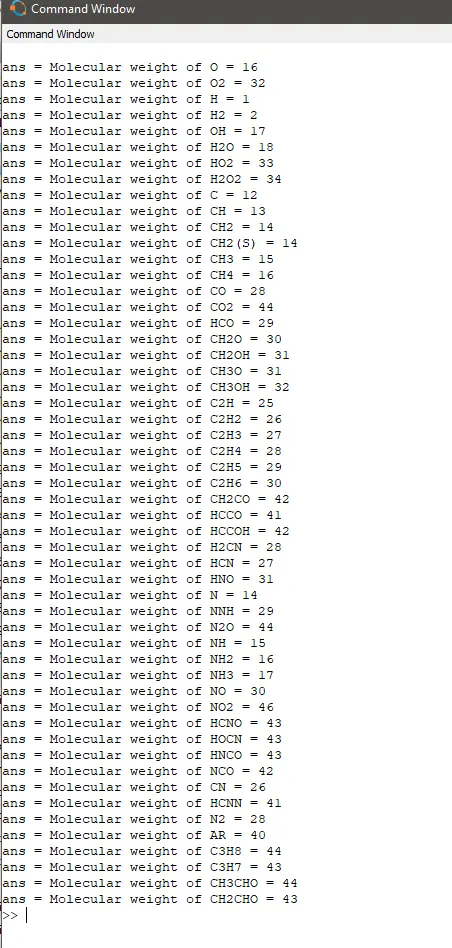

Plot:-

For O2:-

For N2:-

For co2:-

Picture of species folders:

Conclusion:-

• The characteristic curves for all the species are obtained.
• N2 and O2 follow the same general pattern with the only difference being that O2 gives out energy (positive enthalpy) and N2 takes in energy (negative enthalpy). Their relation to Temperature is as expected as they follow a parabolic path for Cp and S and a linear plot for H since Cp and S are inversely proportional to temperature and H is directly proportional to it.