Project 1 - Parsing NASA thermodynamic data

Parsing in computer languages refers to the syntactic analysis of the input code into its components parts in order to facilitate the writing of compilers and interpreters. It can be used to describe split or separation.

Parsing a file means reading in a data stream of some sort and building an in-memory model of the semantic content of that data. This aims at facilitating performing some kind of transformation on the data.

The file is provided is NASA libraries of thermodynamic data and transport properties are given for individual species in the form of least-squares coefficients. Values of heat capacity Cp(T), enthalpy H°(T), and entropy S°(T) are available for 1130 solid, liquid, and gaseous species. Viscosity and thermal conductivity data are given for 155 gases. The original Cp(T) values were
fit to a fourth-order polynomial with integration constants for H°(T) and S°(T). For each species the integration constant. for H°(T) includes the heat of formation. Transport properties have a different functional form. The temperature range for most of the data is 300 to 5000 K, although some of the newer thermodynamic data have a range of 200 to 6000 K. Because the species are mainly possible products of the reaction, the data are useful for chemical equilibrium and kinetics computer codes. Much of the data has been distributed for several years with the NASA Lewis equilibrium program CET89. The thermodynamic properties of the reference elements have been updated along with about 175 species that involve the elements carbon, hydrogen, oxygen, and nitrogen. These sets of data will be distributed with the NASA Lewis personal computer program for calculating chemical equilibria, CETPC.

In this project, the aim is to extract these coefficients from the file. here only a part of the data is taken since it is for example. Coefficients extracted to be used to calculate the Specific heat, Enthalpy and Entropy using the below formulas as figure 1 shows.

Code:-

The code is divided into 5 sections, these sections are to calculate the specific heat, enthalpy, entropy, plotting and calculating the molecular weight of the element.

The main code is shown in figure 2.

% Project: File Parsing of NASA Thermodynamic Data
% Done by Murtadha Zainy 

close all
clear
clc
 
%GasConstant Value
R= 8.314; 
 
%Reading the data file given 
f1 = fopen('THERMO.dat','r');
 
%Reading the first line of the file 
fgetl(f1);
 

Global_temp = fgetl(f1);
t = strsplit(Global_temp);
global_min = str2double(t{2});
global_mid = str2double(t{3});
global_max = str2double(t{4});

%Defining the temperature range
temp = linspace (global_min,global_max,500);
 

for i=1:3
fgetl(f1);
end


for i=1:53
    % the first line which includes the information for species
    l=fgetl(f1);   
 
    
    element_name=strtok(l);
 
    l1=fgetl(f1);
    l2=fgetl(f1);
    l3=fgetl(f1);
    
    %Finding the position of E in each given temperature
    P1=strfind(l1,'E');
    P2=strfind(l2,'E');
    P3=strfind(l3,'E');
 
%finding the high temperature coefficient
    hc1=str2double(l1(1:P1(1)+3));
    hc2=str2double(l1(P1(1)+3:P1(2)+3));
    hc3=str2double(l1(P1(2)+4:P1(3)+3));
    hc4=str2double(l1(P1(3)+4:P1(4)+3));
    hc5=str2double(l1(P1(4)+4:P1(5)+3));
    hc6=str2double(l2(1:P2(1)+3));
    hc7=str2double(l2(P2(1)+4:P2(2)+3));
 
%finding the low temperature coefficient
    lc1=str2double(l2(P2(2)+4:P2(3)+3));
    lc2=str2double(l2(P2(3)+4:P2(4)+3));
    lc3=str2double(l2(P2(4)+4:P2(5)+3));
    lc4=str2double(l3(1:P3(1)+3));
    lc5=str2double(l3(P3(1)+4:P3(2)+3));
    lc6=str2double(l3(P3(2)+4:P3(3)+3));
    lc7=str2double(l3(P3(3)+4:P3(4)+3));
 
 %Calling the specific heat function
    c_p = specific_heat(hc1,hc2,hc3,hc4,hc5,lc1,lc2,lc3,lc4,lc5,R,temp,global_mid);
 
    %Calling the enthalpy function
    H = enthalpy(hc1,hc2,hc3,hc4,hc5,hc6,lc1,lc2,lc3,lc4,lc5,lc6,R,temp,global_mid);
 
    %Calling the entropy function
    S = entropy(hc1,hc2,hc3,hc4,hc5,hc7,lc1,lc2,lc3,lc4,lc5,lc7,R,temp,global_mid);
    
    %Calling the Plotting function
 s   plotting(c_p,H,S,temp,element_name);
 
    
    %Calculating the molecular weight function 
    mw(i) = molecular_weight(element_name); 
    X=sprintf('%s_%d',element_name,mw(i));
    disp(X);
    
end
fclose(f1)

Before writing the code, it's important to start with clear all, close all and clc commands since

Clear all - removes data from the workspace, freeing up system memory

Close all- deletes the current figure or the specified figure

clc - clears all input and output from the Command Window display, giving you a "clean screen".

Next step is to define the constants, R which is the gas constant has been defined as 8.314.

The next step is to open and read the file text given, the fopen command is used to open the file. fgetl command was used to return the next line of the specified file, removing the newline characters since the first line is not required for this project . then the second line which contains the global temperature ranges was stored in 3 variables,'global_min','global_max','global_mid'. Then, an array for temperature is defined which contains 500 different values between global min and global max. a for loop was made to ignore the 3 next comments in the file. The temperature coefficients of 53 species were defined using a for loop, strtok command was used to read the first character of the element name.

The subsequent three lines contain the 14 different coefficients(high and low), which were first stored in 3 variables. The position of E had to be found out to move to the next value. After finding out the positions of E for each temperature, the next step was to find out the high and low-temperature coefficients. Str2double command converts the text in str to double-precision values. str contains text that represents real or complex numeric values. str can be a character vector, a cell array of character vectors, or a string array. If str is a character vector or string scalar, then X is a numeric scalar. If str is a cell array of character vectors or a string array, then X is a numeric array that is the same size as str.

After calculating the high and low-temperature coefficients, four separate functions are written specifically to calculate, Specific Heat, Enthalpy, Molecular weight and Entropy. After calculating the variables a plot function was used to plot several graphs.

Finally, the file is closed by using the close command.

Specific Heat Function:-

Figure 3 shows the code for specific heat function

function [c_p] = specific_heat(a1,a2,a3,a4,a5,b1,b2,b3,b4,b5,R,temp,global_mid)

    if temp<=global_mid
       c_p = R*(a1 + a2.*temp + a3.*(temp.^2) + a4.*(temp.^3) + a5.*(temp.^4));
    else
        c_p = R*(b1 + b2.*temp+b3.*(temp.^2) + b4.*(temp.^3) + b5.*(temp.^4));
end

The variables of this function were, the first 5 low and high coefficients, temperature, R gas constant and global mid-temperature function. The global mid-temperature is used to define the condition whether the temperature of the element is lower than or greater than it so then the appropriate low or high temper. The condition was checked by an if-else condition.

Enthalpy Function:-

Figure 4 shows the code for enthalpy function

 
function [H] = enthalpy(a1,a2,a3,a4,a5,a6,b1,b2,b3,b4,b5,b6,R,temp,global_mid)
    if temp <=global_mid
        H = R.*temp.*(a1 + a2.*(temp./2) + a3.*((temp.^2)./3) + a4.*((temp.^3)./4)...
            + a5.*((temp.^4)./5) + a6./temp);
    else
        H = R.*temp.*(b1 + b2.*(temp./2) + b3.*((temp.^2)./3) + b4.*((temp.^3)./4)...
            + b5.*((temp.^4)./5) + b6./temp);
        
end 

The variables of this function were, the first 5 low and high coefficients, temperature, R gas constant and global mid-temperature function. The global mid-temperature is used to define the condition whether the temperature of the element is lower than or greater than it so then the appropriate low or high temper. The condition was checked by an if-else condition.

Entropy Function:-

Figure 5 shows the code for entropy function

function [S] = entropy(a1,a2,a3,a4,a5,a7,b1,b2,b3,b4,b5,b7,R,temp,global_mid)
    if temp<=global_mid
        S = R*(a1.*log(temp) + a2.*temp + a3.*(temp.^2)./2 + a4.*(temp.^3)./3 + a5.*(temp.^4)./4 + a7);
   else
        S = R*(b1.*log(temp) + b2.*temp + b3.*(temp.^2)./2 + b4.*(temp.^3)./3 + b5.*(temp.^4)./4 + b7);
 
 end

The variables of this function were, the first 5 low and high coefficients, temperature, R gas constant and global mid-temperature function. The global mid-temperature is used to define the condition whether the temperature of the element is lower than or greater than it so then the appropriate low or high temper. The condition was checked by an if-else condition.

Molecular Weight:-

Figure 6 shows the code for molecular weight function

function [weight] = molecular_weight(element_name)
 
s = {'H' 'C' 'N' 'O' 'AR'};
 
%atomic weight of each elements
atomic_wt = [1 12 14 16 40];                                               
weight = 0;                                                                        
 
for i = 1:length(element_name) 
for j = 1:length(s)   
if strcmp(element_name(i), s(j)) 
 weight= weight + atomic_wt(j);     
 
%storing the position of matched element  
pos = j;                                                           
 
end
 
end    
 
n = str2double(element_name(i));
if n > 1                                               
weight = weight + atomic_wt(pos)*(n-1); 
 
end
 
end
 
end

This function only takes the element name as the input variable. First, a string is created with the 5 basic element names , along with that an atomic weight function which contains their atomic weights. Then used 'strcmp' command to compare the name of the element with the string array. If there is a repetition of an element, 'str2double' is used to find that and (n-1) is multiplied to atomic_wt of the element to calculate the molecular weight of the respective species.

Plotting Function:-

Figure 7 shows the code for plotting function

function plotting(c_p,H,S,temp,element_name)

cd(pwd);                
dir_name=element_name;


mkdir(dir_name);
 
 %Plotting temperature vs specific heat 
figure(1)
plot(temp,c_p,'lineWidth',3,'color','r');
title(sprintf('Specific Heat vs Temperature for %s:',element_name));
xlabel('Temperature');
ylabel('Specific Heat'); 
 
% Plotting temperature vs Enthalpy
figure(2)
plot(temp,H,'linewidth',3,'color','g');
title(sprintf('Enthalpy vs Temperature for %s:',element_name));
xlabel('Temperature');
ylabel('Enthalpy'); 
 
% Plotting temperature vs Entropy
figure(3)
plot(temp,S,'linewidth',3,'color','b');
title(sprintf('Entropy vs Temperature for %s:',element_name));
xlabel('Temperature');
ylabel('Entropy'); 
cd(dir_name);

%To save the images captured
saveas(1,'c_p_vs_temp.png');
saveas(2,'H_vs_temp.png');
saveas(3,'S_vs_temp.png'); 
 
cd .. ;
 
end

This Function requires all the variables we have mentioned prior. the cd(pwd) command was used to store the data in the current directory, the mkdir command was used to make a new file for the next study.

Next step is to plot, three plot types were used. Temperature vs specific heat, temperature vs enthalpy and finally temperature vs entropy. Plots were saved using the save as command and each element had 3 different plots that were stored in a file.

Results:-

Figure 8 shows the molecular weight for each element

O_16
O2_32
H_1
H2_2
OH_17 
H2O_18
HO2_33
H2O2_34
C_12 
CH_13
CH2_14
CH2(S)_14
CH3_15 
CH4_16
CO_28 
CO2_44
HCO_29
CH2O_30
CH2OH_31
CH3O_31
CH3OH_32
C2H_25
C2H2_26
C2H3_27
C2H4_28
C2H5_29
C2H6_30
CH2CO_42
HCCO_41
HCCOH_42
H2CN_28
HCN_27
HNO_31
N_14
NNH_29
N2O_44
NH_15
NH2_16
NH3_17
NO_30
NO2_46
HCNO_43
HOCN_43
HNCO_43
NCO_42
CN_26
HCNN_41
N2_28
AR_0
C3H8_44
C3H7_43
CH3CHO_44
CH2CHO_43
C3H8_44
C3H7_43
CH3CHO_44
CH2CHO_43

Figure 9 shows the file locations for each element

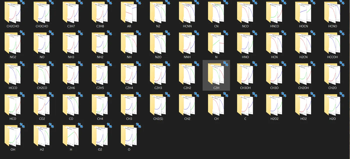
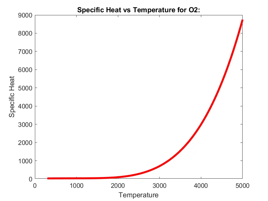
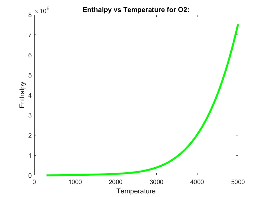
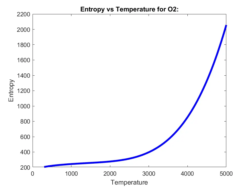
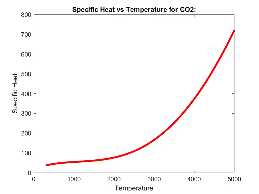
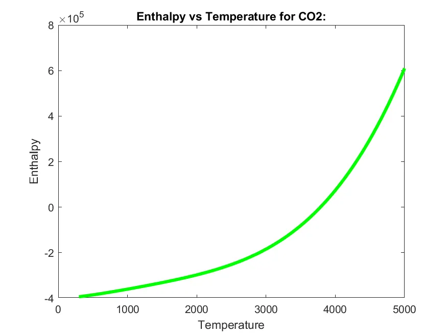
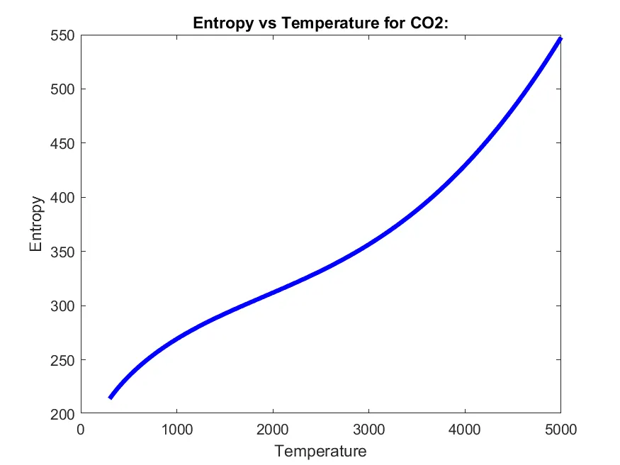
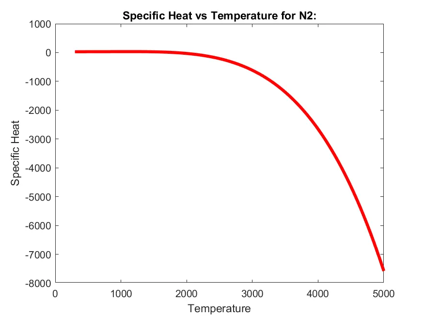
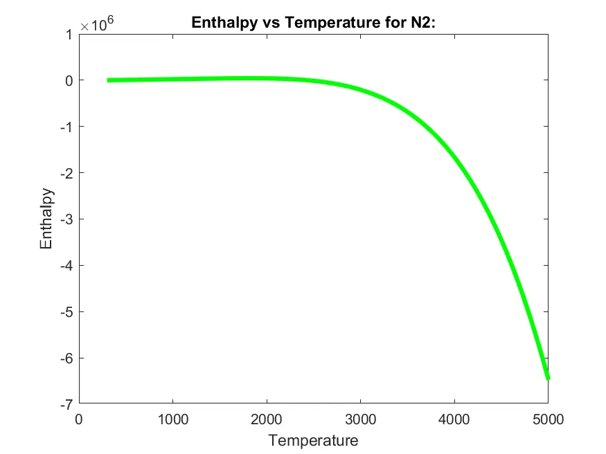
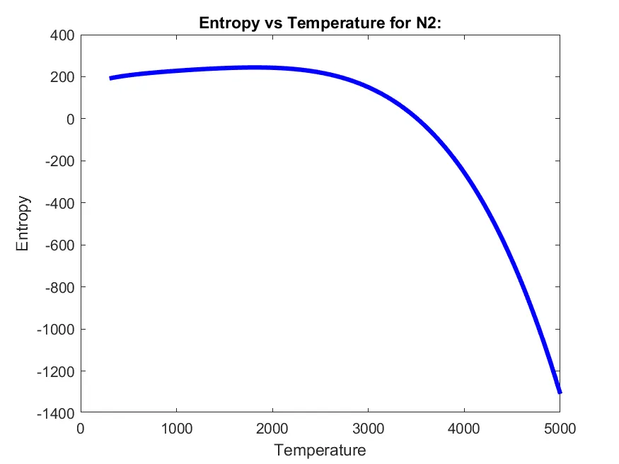
Figure 10,11,12 shows plots for O2. 13,14,15 for CO2 and 16,17,18 for N2