Project 1 - Parsing NASA thermodynamic data

Answer:

THEORY :

Parsing is the process of analyzing a string of symbols, either in natural language, computer languages or data structure, conforming to the rules of formal grammar. The term Parsing comes from the Latin word 'Pars' meaning 'Part'.

In this project, we are going to parse NASA's thermodynamic data and evaluate its thermodynamic properties such as Cp, H and S for all the species given in the data file.

The formulae we are using are given below:

         

where,

          Cp - Specific Heat (kJ/kg K)

           R  - Universal Gas Constant (kJ/kg K)

           H  - Enthalpy (kJ/kg)

           T  - Temperature (K)

           S  - Entropy (kJ/K)

Specific Heat of a Gas at Constant Pressure (Cp) -

It is defined as the amount of heat energy required to raise the temperature of the unit mass of gas by one degree at constant pressure. As per the above formula

               `Cp = R*[a_1 + a_2*T + a_3 *T^2 + a_4*T^3 + a_5*T^4]`

Enthalpy (H) - 

Enthalphy is the property of a gas which is equal to algebraic sum of internal energy and the product of pressure and volume. As per above formula

               `H = (R*T)*[ a_1 + a_2 *(T/2) + a_3*((T^2)/3) + a_4*((T^3)/4) + a_5*((T^4)/5 ) + a_6/T]`

Entropy (S) - 

Entropy is a property of a thermodynamic system that expresses the direction or outcome of spontaneous changes in the system. It predicts that certain processes are irreversible or impossible, despite not violating the conservation of energy. As per the above formula

               `S = R*[ a_1*log(T) + a_2 *T+ a_3*((T^2)/2) + a_4*((T^3)/3) + a_5*((T^4)/4 ) + a_7]`

MATLAB Program:

% MATLAB Program for Parsing the NASA's thermodynamic data
clear all
close all
clc

% Step I : Given
% Universal Gas Constant (kJ/kg K)
R = 8.31446;

% Reading NASA's Thermodynamic Data File
f1 = fopen('THERMO.dat', 'r');
fgetl(f1);

% Step II : Defining Global Temperatures
% Converting strings into numeric value
templ = str2num(fgetl(f1));
low_temp = templ(1);
mid_temp = templ(2);
high_temp = templ(3);

% Step III : Skipping Unwanted Lines
for i = 1:3
    fgetl(f1);
end

% Step IV : Global Temperature Range
T = linspace(low_temp, high_temp, 1000);

% Step V : Extracting First 7 Higher & Second 7 Lower Temperature Coefficients
for j = 1:53
    l_str = fgetl(f1);
    l = strsplit(l_str, ' ');
    m = length(l);
    species = l{1};

    % Storing the values of 1st Line
    l1_str = fgetl(f1);

    % Finding Position of E
    a = strfind(l1_str, 'E');
    
    % Reading all the variable and convert
    a1  = str2num(l1_str(1:a(1)+3));
    a2  = str2num(l1_str((a(1)+4):(a(2)+3)));
    a3  = str2num(l1_str((a(2)+4):(a(3)+3)));
    a4  = str2num(l1_str((a(3)+4):(a(4)+3)));
    a5  = str2num(l1_str((a(4)+4):(a(5)+3)));

    % Storing the values of 2nd Line
    l2_str = fgetl(f1);

    % Finding Position of E
    b = strfind(l2_str, 'E');

    % Reading all the variable and convert
    a6  = str2num(l2_str(1:b(1)+3));
    a7  = str2num(l2_str((b(1)+4):(b(2)+3)));
    a8  = str2num(l2_str((b(2)+4):(b(3)+3)));
    a9  = str2num(l2_str((b(3)+4):(b(4)+3)));
    a10 = str2num(l2_str((b(4)+4):(b(5)+3)));
    
    % Storing the values of 2nd Line
    l3_str = fgetl(f1);

    % Finding Position of E
    c = strfind(l3_str, 'E');
    
    % Reading all the variable and convert
    a11 = str2num(l3_str(1:c(1)+3));
    a12 = str2num(l3_str((c(1)+4):(c(2)+3)));
    a13 = str2num(l3_str((c(2)+4):(c(3)+3)));
    a14 = str2num(l3_str((c(3)+4):(c(4)+3)));
   
    % Step VI : Calculate Specific Heat, Enthalpy & Entropy 
    % if-else statement to find values of Cp, h and S at different Temperature

if T < mid_temp
    Cp = R.*(a1 + a2.*T + a3.*(T.^2) + a4.*(T.^3) + a5.*(T.^4));
    h  = (R.*T).*(a1 + a2.*(T./2) + a3.*((T.^2)./3) + a4.*((T.^3)./4) + a5.*((T.^4)./5) + (a6./T));
    S  = R.*(a1.*log(T) + a2.*T + a3.*((T.^2)./2) + a4.*((T.^3)./3) + a5.*((T.^4)./4) + a7);

else
    Cp = R.*(a8 + a9.*T + a10.*(T.^2) + a11.*(T.^3) + a12.*(T.^4));
    h  = (R.*T).*(a8 + a9.*(T./2) + a10.*((T.^2)./3) + a11.*((T.^3)./4) + a12.*((T.^4)./5) + (a13./T));
    S  = R.*(a8.*log(T) + a9.*T + a10.*((T.^2)./2) + a11.*((T.^3)./3) + a12.*((T.^4)./4) + a14);
end

% Step VII : Calculating Molecular Weight of each Species
W = molecular_weight(species);

mw_file = fopen('molecular_weight.txt', 'w');
fprintf(mw_file,'molecular_weight of %s is %d', species);
fclose(mw_file);

% Step VIII : Creating NASA's Thermodynamic Data for each Species
cur_dir = pwd;
mkdir(species);
cd(species);

% Step IX : Plotting Specific Heat, Enthalphy and Entrophy with Temperature

% Plot Specific Heat (Cp) vs Temperature (T)
figure(1)
plot(T, Cp, 'LineWidth',3,'Color','r');
xlabel('Temperature (K)')
ylabel('Specific Heat (kJ/kg K)');
title(sprintf('Specific Heat vs Temperature range of %s', species));
saveas(figure(1), 'Specific Heat.jpg');
grid on

% Plot Enthalphy (h) vs Temperature (T)
figure(2)
plot(T, h, 'LineWidth',3,'Color','g');
xlabel('Temperature (K)')
ylabel('Enthalphy (kJ/kg)');
title(sprintf('Enthalphy vs Temperature range of %s', species));
saveas(figure(2), 'Enthalphy.jpg');
grid on

% Plot Entrophy (S) vs Temperature (T)
figure(3)
plot(T, Cp, 'LineWidth',3,'Color','b');
xlabel('Temperature (K)')
ylabel('Entrophy (kJ/K)');
title(sprintf('Entrophy vs Temperature range of %s', species));
saveas(figure(3), 'Entrophy.jpg');
grid on

cd(cur_dir);

Explanation

• The universal gas constant value R is 8.31446 kJ/kg K. Later we have opened the given ’Thermo.dat’ file by using fopen command with an instruction ‘r’ for reading the file.
• We have defined the temperatures as low, medium and high. Next, we have converted the data which is in a string value to a numeric value by using ’str2num’ command.
• As first few lines of the data were not required. So we have skipped those unwanted lines by using for loop command.
• We have used linspace command which gives the start to end value with several elements in it.
• Here we have formulated a program to extract all the 14 coefficients which have the first 7 higher and next 7 lower temperature coefficients with the help of for loop command by finding the position of E using strfind. Once the place value of E is known then we extracted all the variables and converted them into numeric using ‘str2num’ command.
• Here we have calculated the values of Cp, h & S using the given formula with T.
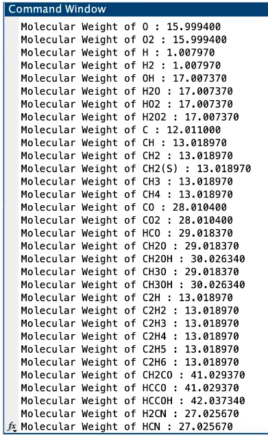
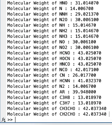
• Molecular weights are calculated using function W for each species and created a text file that has the result. Later program in such a way that its result is shown in the command window once it is recalled at the end.
• Once, all the data runs properly then data will be stored in the desired file based on their species.
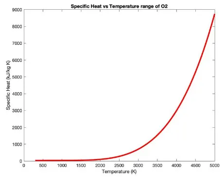
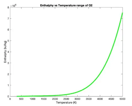
• As Cp, h, & S are known, the plot commands help to plot graphs for each species and save them in jpg format using saveas command.

Functional Program:

function W = molecular_weight(species)

% Step I : Atomic Names
% Hydrogen (H), Carbon (C), Nitrogen (N), Oxygen (O) and Argon (Ar)
atoms = ['H', 'C', 'N', 'O', 'Ar'];

% Step II : Atomic Weight
atomic_weight = [1.00797 12.011 14.0067 15.9994 39.948];

% Step III : Starting Molecular Range
W = 0;
for i = 1:length(species)
    for j = 1:length(atoms)
        if strcmp(species(i), atoms(j))
            W = W + atomic_weight(j);
            position = j;
        end
    end
% Step IV : Finding Molecular Weight for more Species
    n = str2num(species);
    if n > 1
        W = W + (atomic_weight(position).* (n-1));
    end
end

% Step V : Results
fprintf('Molecular Weight of %s : ', species);
fprintf('%f', W);
disp(' ');
end

RESULTS :

Molecular Weight of Species

     

      

Output:

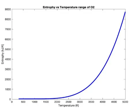
Graphs of O2:

                    

                                                                  

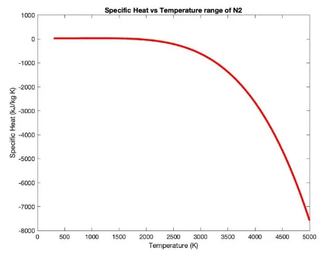
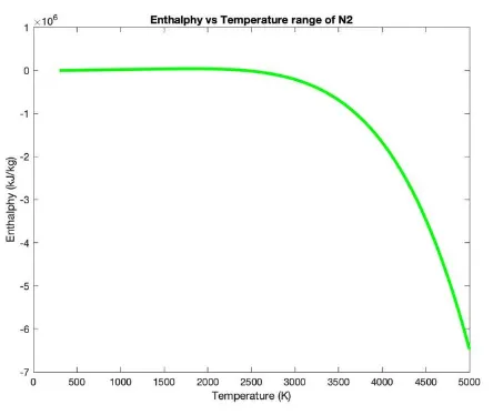
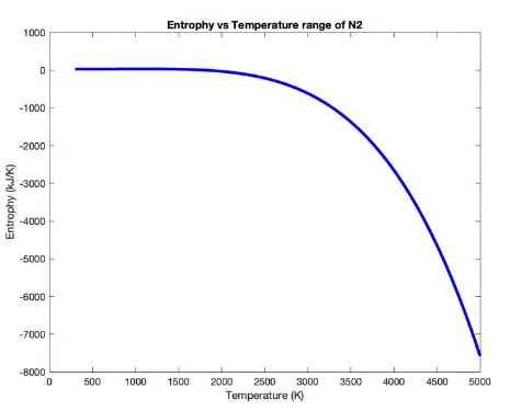
Graphs of N2:

                 

                                                               

Graphs of CO2:

               

                                                                 

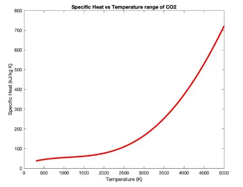
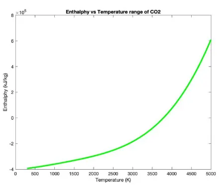
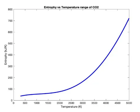
CONCLUSION :

By using MATLAB, we have obtained the temperature coefficients for high and low temperatures relative to their local temperature ranges. The specific heat, enthalpy and entropy of all species are calculated concerning their given formula, and graphs are drawn. Also, the molecular weights are calculated and displayed in the command window.