Project 1 - Parsing NASA thermodynamic data
Parsing NASA thermodynamic data
AIM:
- To write a program in MatLab to parse the NASA thermodynamic data file and then calculate the thermodynamic properties of various gas species.
OBJECTIVE:
- To write a function that extracts the 14 co-efficient and calculates the enthalpy, entropy, and specific heats for all species in the data file.
- Calculating the molecular weight of each species and displaying it in the command window.
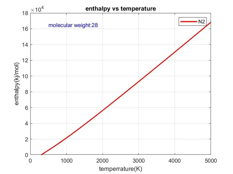
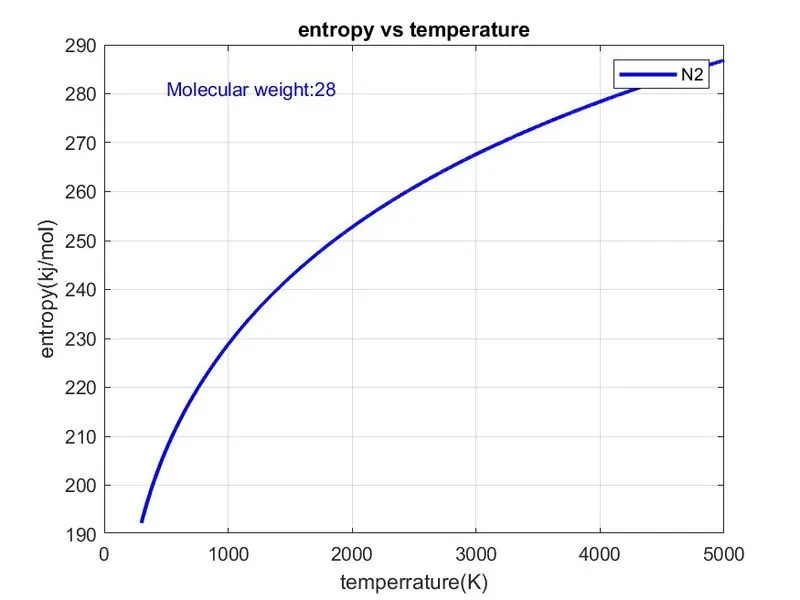
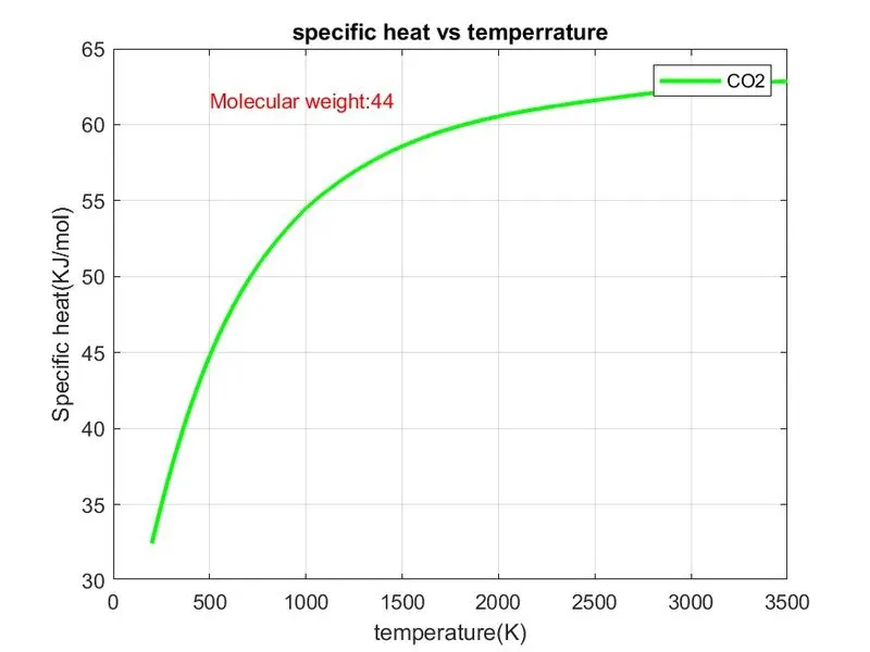
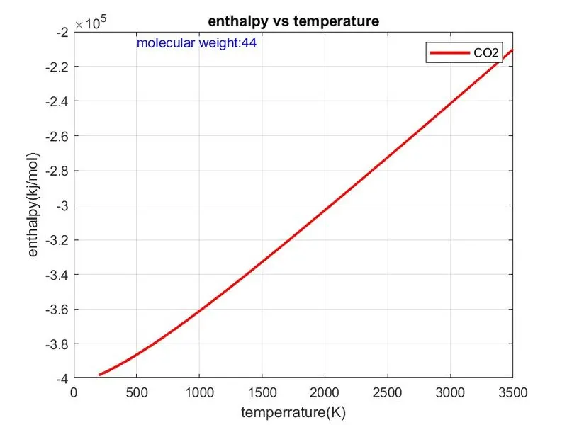
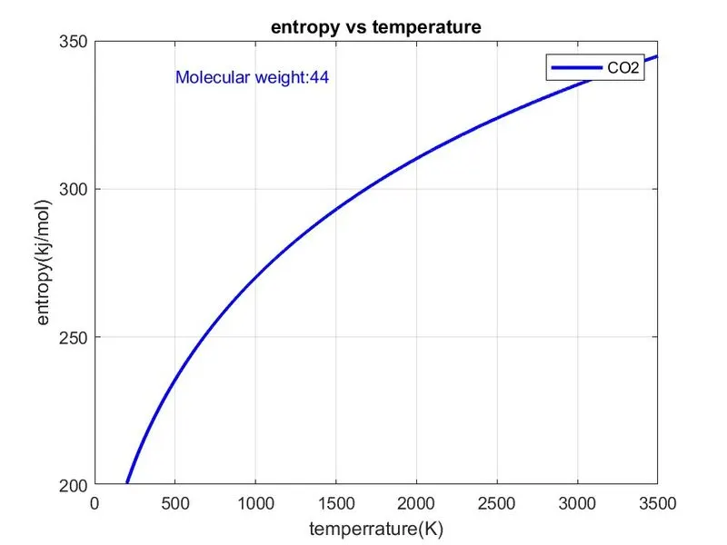
- Plotting cp, enthalpy, and entropy for local temperature range specified for each species.
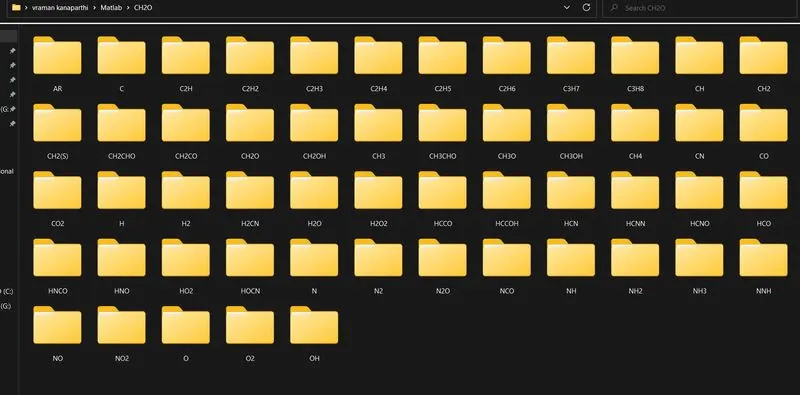
- Save the plot as images with appropriate names and dump them in separate folders for each species with a suitable name.
INTRODUCTION:
PARSING DATA:
- Parsing means to make something understandable. For programming, this means converting information represented in one form into another form that's easier to work with. This is done by partially analyzing the data, understanding its underlying structure (by making some assumptions based on what you're expecting to see), and then explicitly representing that structure in the code.
- Parsing a file means reading in a data stream of some sort and building an in-memory model of the semantic content of that data. This aims at facilitating performing some kind of transformation on the data.
EQUATIONS:
The equations that we are going to use in the Functions to calculate cp, H, and S are:
Where,
- Cp = specific heat
- R = molar gas constant
- T = temperature
- S = Entropy
- H = Enthalpy
- a = coefficients
PROGRAM:
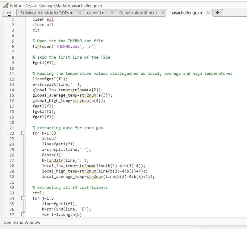
clear all
close all
clc

% Open the the THERMO.dat file
f1=fopen('THERMO.dat', 'r')

% skip the first line of the file
fgetl(f1);

% Reading the tempersture values distingushed as local, average and high temperatures
line=fgetl(f1);
a=strsplit(line,' ');
global_low_temp=str2num(a{2});
global_average_temp=str2num(a{3});
global_high_temp=str2num(a{4});
fgetl(f1);
fgetl(f1);
fgetl(f1);

% extracting data for each gas
for k=1:53
    %step7
    line=fgetl(f1);
    a=strsplit(line,' ');
    Gas=a(1);
    b=findstr(line,'.');
    local_low_temp=str2num(line(b(1)-4:b(1)+4));
    local_high_temp=str2num(line(b(2)-4:b(2)+4));
    local_average_temp=str2num(line(b(3)-4:b(3)+4));

% extracting all 14 coefficients
ct=1;
for j=1:3
    line=fgetl(f1);
    b=strfind(line, 'E');
    for i=1:length(b)
        if ct<=7
            Ha(ct)=str2num(line(b(i)-11:b(i)+3));
            ct=ct+1;
        else
            La(ct-7)=str2num(line(b(i)-11:b(i)+3));
            ct=ct+1;
        end
    end
end

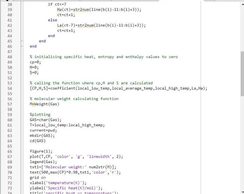
% initializing specific heat, entropy and enthalpy values to zero
cp=0;
H=0;
S=0;

% calling the function where cp,H and S are calculated
[CP,H,S]=coefficient(local_low_temp,local_average_temp,local_high_temp,La,Ha);

% molecular weight calculating function
M=Weight(Gas)

%plotting
GAS=char(Gas);
T=local_low_temp:local_high_temp;
current=pwd;
mkdir(GAS);
cd(GAS)

figure(1);
plot(T,CP, 'color', 'g', 'linewidth', 2);
legend(Gas);
txt1=['Molecular weight:' num2str(M)];
text(500,max(CP)*0.98,txt1,'color','r');
grid on
xlabel('temperature(K)');
ylabel('Specific heat(KJ/mol)');
title('specific heat vs temperrature');

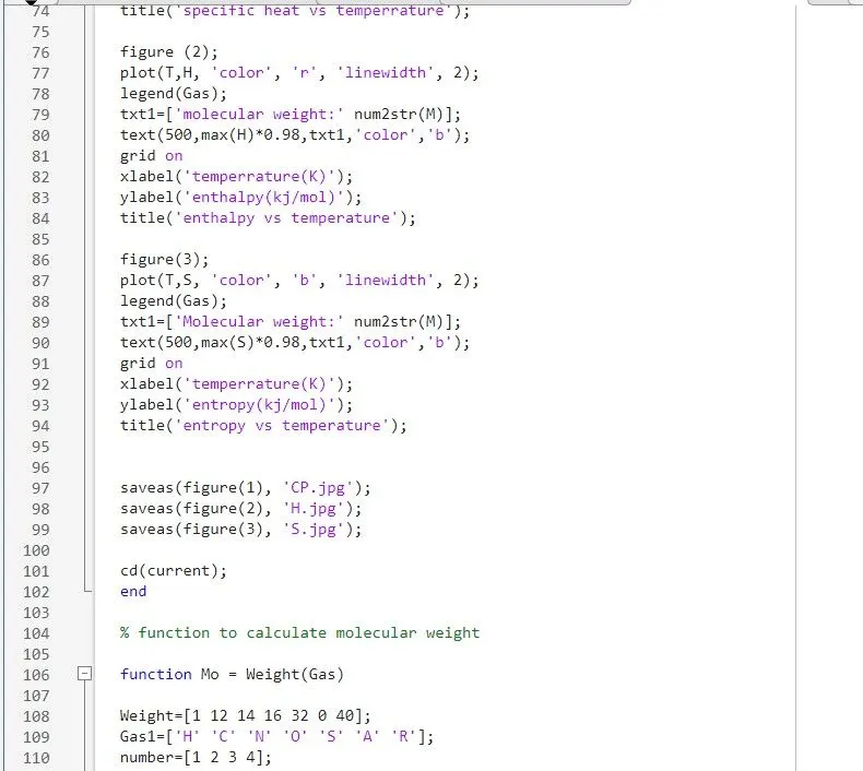
figure (2);
plot(T,H, 'color', 'r', 'linewidth', 2);
legend(Gas);
txt1=['molecular weight:' num2str(M)];
text(500,max(H)*0.98,txt1,'color','b');
grid on
xlabel('temperrature(K)');
ylabel('enthalpy(kj/mol)');
title('enthalpy vs temperature');

figure(3);
plot(T,S, 'color', 'b', 'linewidth', 2);
legend(Gas);
txt1=['Molecular weight:' num2str(M)];
text(500,max(S)*0.98,txt1,'color','b');
grid on
xlabel('temperrature(K)');
ylabel('entropy(kj/mol)');
title('entropy vs temperature');


saveas(figure(1), 'CP.jpg');
saveas(figure(2), 'H.jpg');
saveas(figure(3), 'S.jpg');

cd(current);
end

% function to calculate molecular weight

function Mo = Weight(Gas)

Weight=[1 12 14 16 32 0 40];
Gas1=['H' 'C' 'N' 'O' 'S' 'A' 'R'];
number=[1 2 3 4];

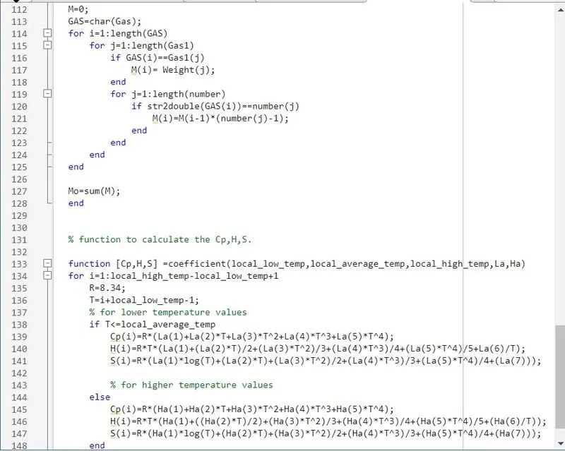
M=0;
GAS=char(Gas);
for i=1:length(GAS)
    for j=1:length(Gas1)
        if GAS(i)==Gas1(j)
            M(i)= Weight(j);
        end
        for j=1:length(number)
            if str2double(GAS(i))==number(j)
                M(i)=M(i-1)*(number(j)-1);
            end
        end
    end
end

Mo=sum(M);
end


% function to calculate the Cp, H, S.

function [Cp,H,S] =coefficient(local_low_temp,local_average_temp,local_high_temp,La,Ha)
for i=1:local_high_temp-local_low_temp+1
    R=8.34;
    T=i+local_low_temp-1;
    % for lower temperature values
    if T<=local_average_temp
        Cp(i)=R*(La(1)+La(2)*T+La(3)*T^2+La(4)*T^3+La(5)*T^4);
        H(i)=R*T*(La(1)+(La(2)*T)/2+(La(3)*T^2)/3+(La(4)*T^3)/4+(La(5)*T^4)/5+La(6)/T);
        S(i)=R*(La(1)*log(T)+(La(2)*T)+(La(3)*T^2)/2+(La(4)*T^3)/3+(La(5)*T^4)/4+(La(7)));

        % for higher temperature values
    else
        Cp(i)=R*(Ha(1)+Ha(2)*T+Ha(3)*T^2+Ha(4)*T^3+Ha(5)*T^4);
        H(i)=R*T*(Ha(1)+((Ha(2)*T)/2)+(Ha(3)*T^2)/3+(Ha(4)*T^3)/4+(Ha(5)*T^4)/5+(Ha(6)/T));
        S(i)=R*(Ha(1)*log(T)+(Ha(2)*T)+(Ha(3)*T^2)/2+(Ha(4)*T^3)/3+(Ha(5)*T^4)/4+(Ha(7)));
    end
end
end

EXPLANATION FOR CODE:
- Initially, the value of 'R' is defined.
- Then we use a command to open the file 'THERMO.dat'.
- Further, we use the 'fgetl' to start reading the lines and after reading the first two lines, from the second line convert the strings to numbers and assign global (low, mid, and high) temperatures.
- Then we have written a command to get the temperature range for calculation and plotting purposes.
- Then again use the 'fgetl' command to go to the next 3 lines and skip it.
- Then we use a for loop to get 53 species and their temperatures (low, mid, high) and the 14 coefficients.
- In the for loop we again use the fgetl command and then the next line is read and from that line, the species name, and the three local temperatures are read and stored.
- Then we use the fgetl command to go to a further line and get the first 7 coefficients and store them. Similarly using the fgetl command we move to the next two lines and get the remaining coefficients.
- Then after getting the 14 coefficients, we use these coefficients and by calling the functions we calculate cp, H, S.
- Further, we use the Molecular weight function and calculate the molecular weight for that species.
- Further, I have used a command to change the directory so that I can save the files at a particular location. After changing the directory have used 'mkdir' to create a new folder with the name of the current species and then a 'cd' command to make mkdir as the current directory.
- Then further we use the plot command to plot temperature vs (cp, enthalpy, entropy).
- In this plotting, we use the figure command to get the three different plots and save as a command to save the figures in the
- Then again we change our directory to again start the loop. So the loop continues to function till we get all the 53 species and then gets terminated.
Errors & Command window Execution:
- I have found some errors and solutions were found during execution.
- Use of the semi-colon(;) in coding results in no output in the command window.
- Here I made a mistake that is instead of a semicolon I used a colon so after changing it I was able to solve the problem

RESULT:
Plots for Oxygen(O2):
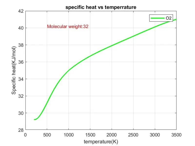
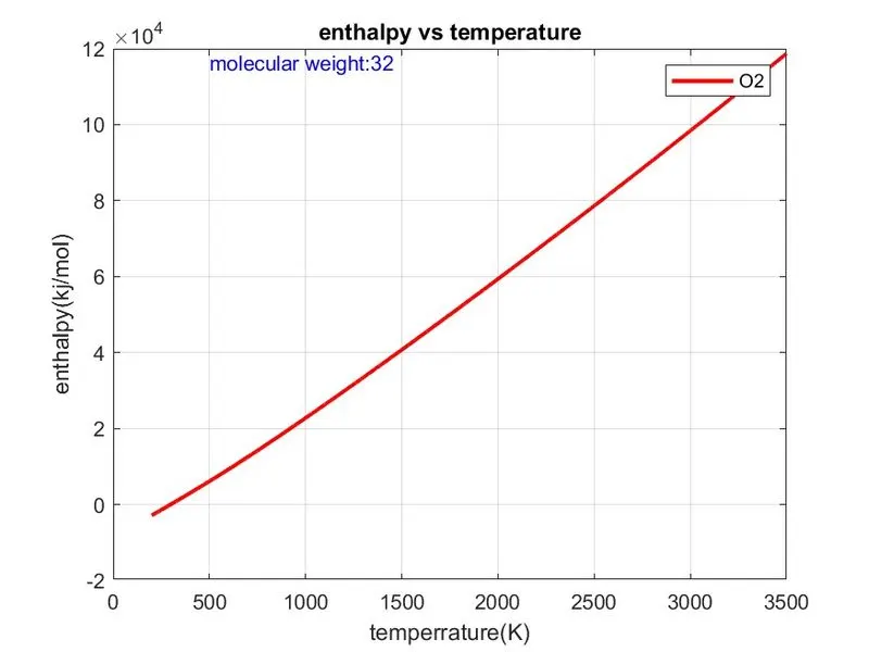
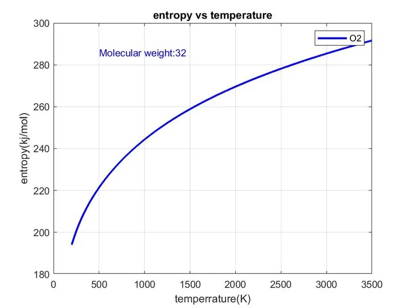
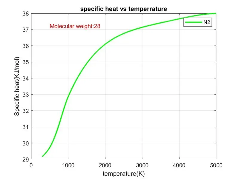
Plots for Nitrogen (N2) :
Plots for Carbon dioxide(Co2) :
SCREENSHOT OF THE FOLDER:
CONCLUSION:
So here we were able to parse the data from the THERMO.dat file. Then using this data we were able to calculate the thermodynamic properties and also make plots for these properties with respect to the temperature.