Project-1: Modelling an electric Car with Li-ion battery

1. Title – MATLAB model of an electric car.

2. Objective –

• To design MATLAB of an electric car with Li-ion battery and DC motor.
• Perform simulation to find status of output velocity with respect to reference velocity.
• To plot for different values of parameter and analyse the plot.

3. Introduction –

Electric vehicle is a vehicle, which uses one or more electric motors for propulsion. Depending type of the vehicle motion may be provided by rotary motor or by linear motor (in tracked vehicle). The electricity stored in battery power the electric motor. Battery can be charged by plugging it in grid, like our phone. According to degree of electricity used, electric vehicle is divided into three categories-BEV, PHEV and HEV.

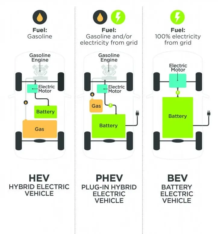
Battery Electric Vehicles (BEV) – BEVs are fully-electric vehicle with rechargeable batteries with no engine. It stores power in battery pack and this power is used to run vehicle and other peripherals. BEVs are charged by electricity from an external source. BEVs don’t emit any hazardous emission. BEVs- Tesla model 3, BMW i3, Kia soul, Toyota Rav4 etc.

Plug-in Hybrid Electric Vehicles (PHEV) – these types of vehicle propelled by motor as well as gasoline engine. Battery is charged with regenerative breaking and it can be charged with external source. PHEVs can go from 10-40miles before assistance of engine. Examples of PHEVs – Chevy volt, Audi A3 E-Tron, BMW i8, Toyota Prius etc.

Hybrid Electric Vehicles (HEV) – HEVs are powered with both gasoline and electricity. Battery can be recharged with regenerative power, only. Motor supplies power for starting and engine take cares at high speed and heavy load. Controller is used to ensure best economy. HEVs – Honda Civic Hybrid, Toyota Prius Hybrid, Toyota Camry Hybrid.

4. Description –

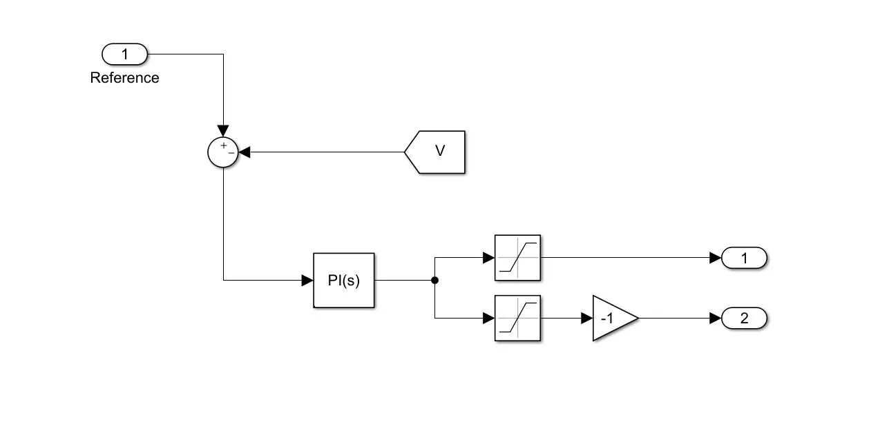
Simulation is an approximation imitation of operations of a system. Simulation is used to get insights of a system. We are going to use Simulink for this project, which is a MATLAB-Based graphical programming environment for modelling, simulating and analysing dynamic system. In this project we are going get insights of an electric vehicle. We will start with modelling subsystems like – electric plant, mechanical plant, controller and then connect them to simulate. We will simulate vehicle for different conditions like presence of wind velocity and grade angle. We will design our own driver block which take reference velocity and feedback and give acceleration and deacceleration command.

Model -

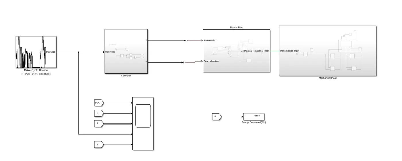
Controller block -

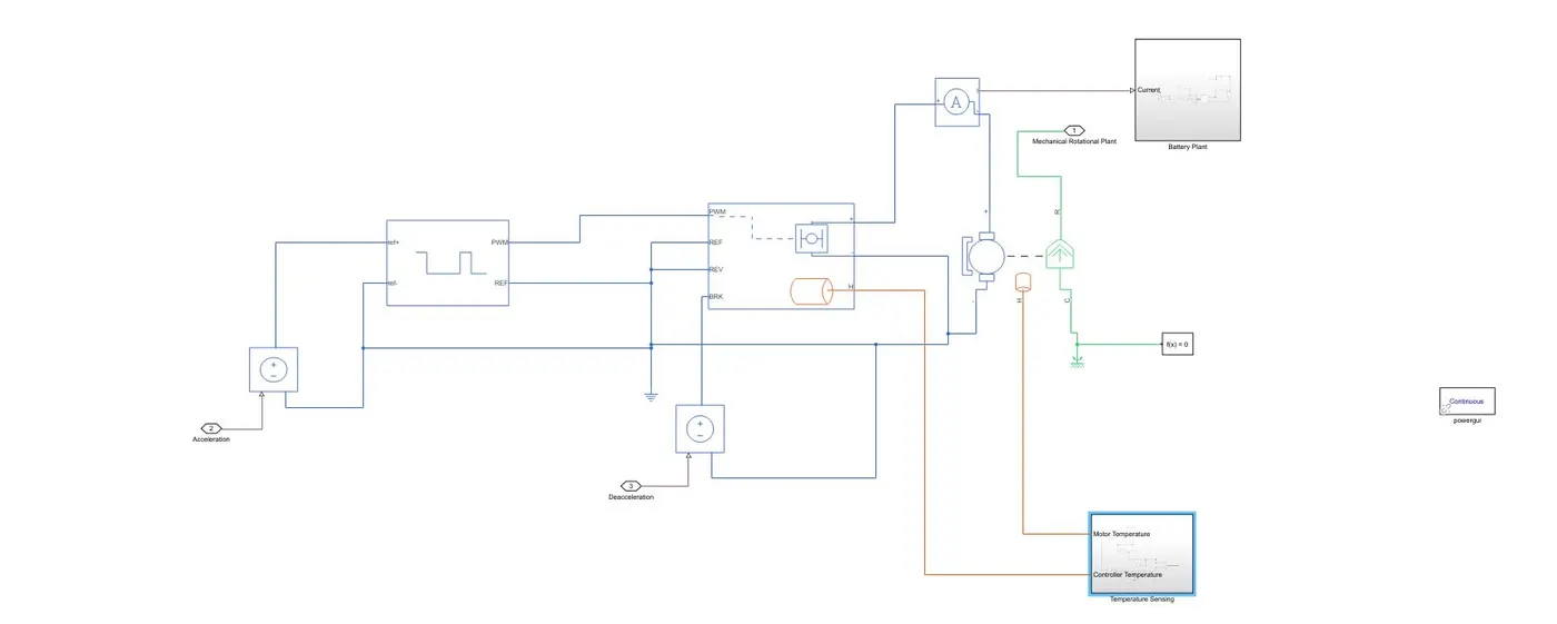
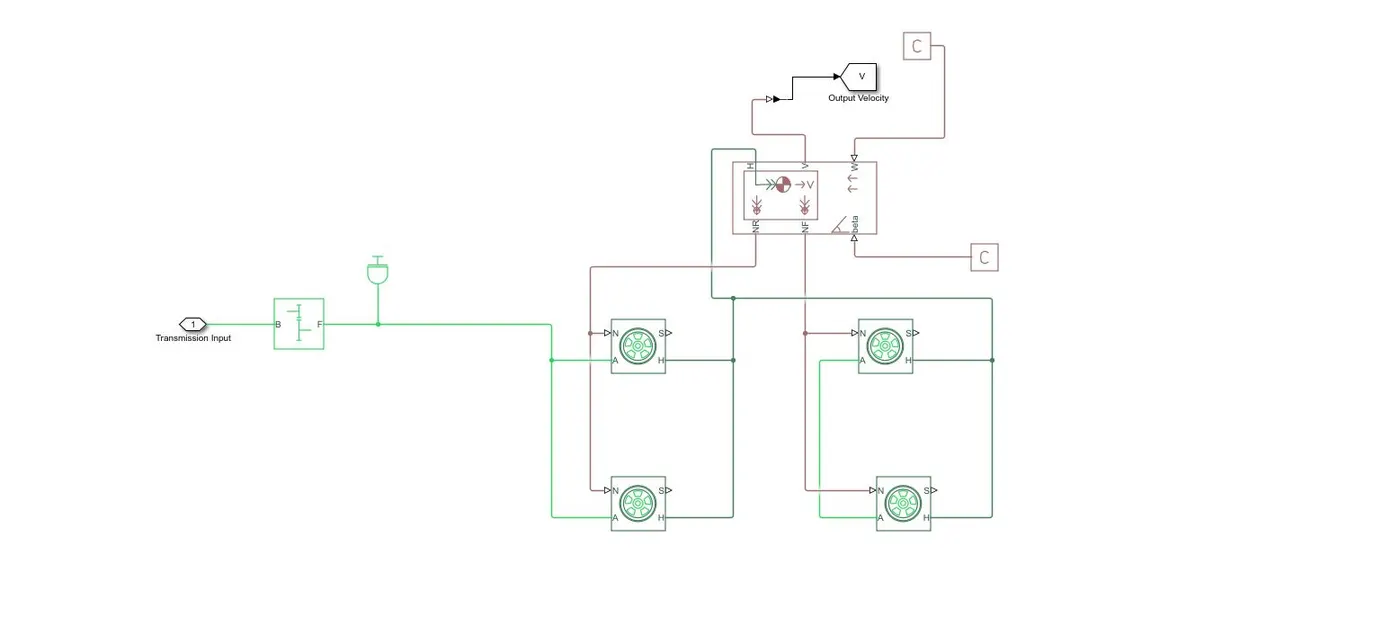
Electric Plant -

Mechanical Plant -

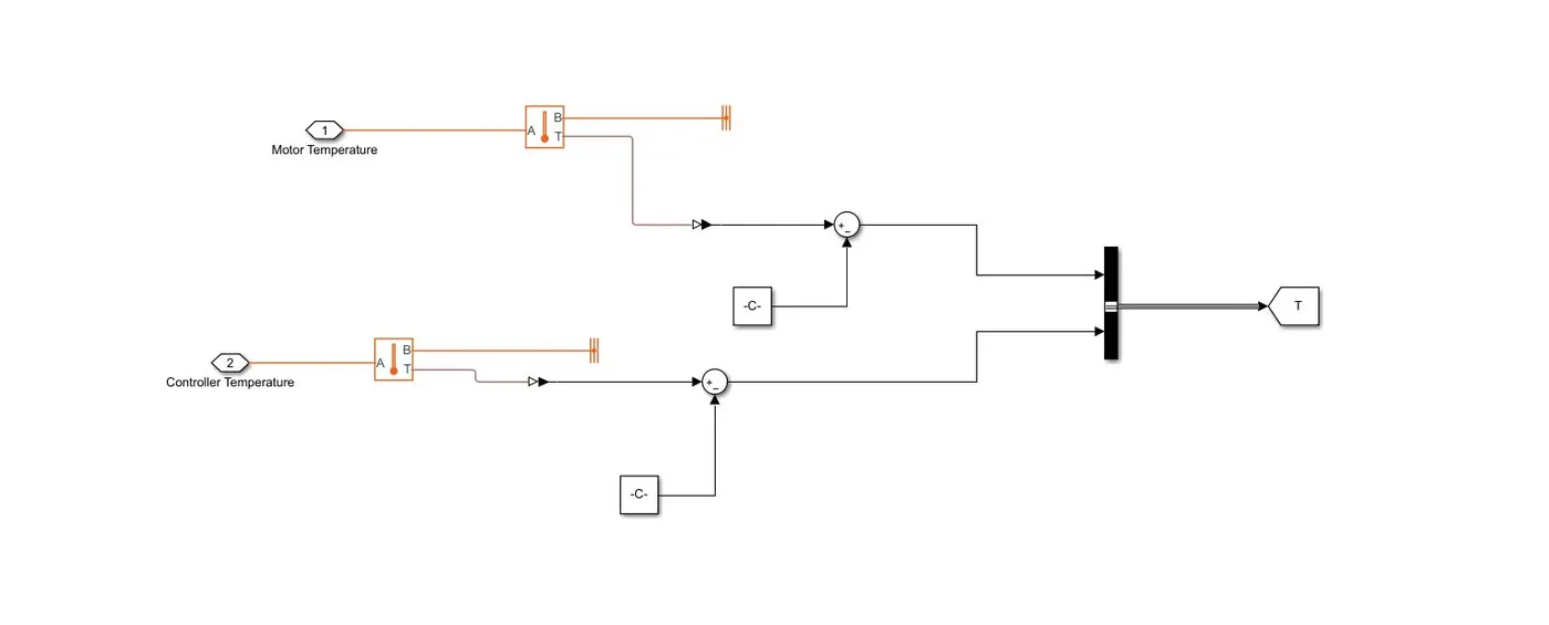
Temperature sensor block -

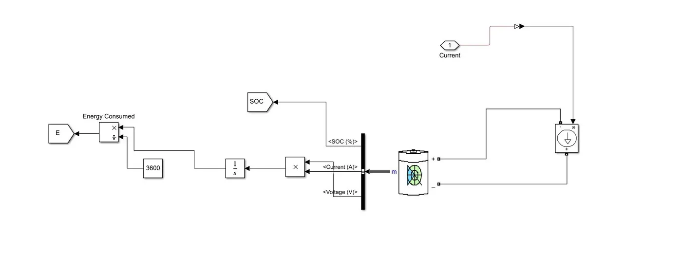
Battery Block -

Blocks used –

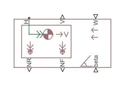
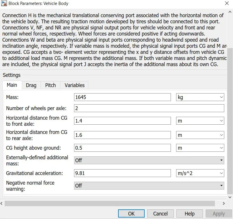
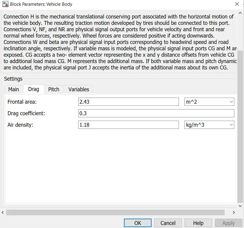
Vehicle body – it represents a vehicle body which have two axle. It has six ports. NR and NF are reserve for normal force. Beta and w are takes grade angle and wind velocity respectively. H represents HUB and connection v gives vehicle velocity. We gave vehicle mass 2126Kg, drag coefficient 0.3, frontal area 2.43.

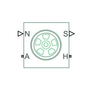
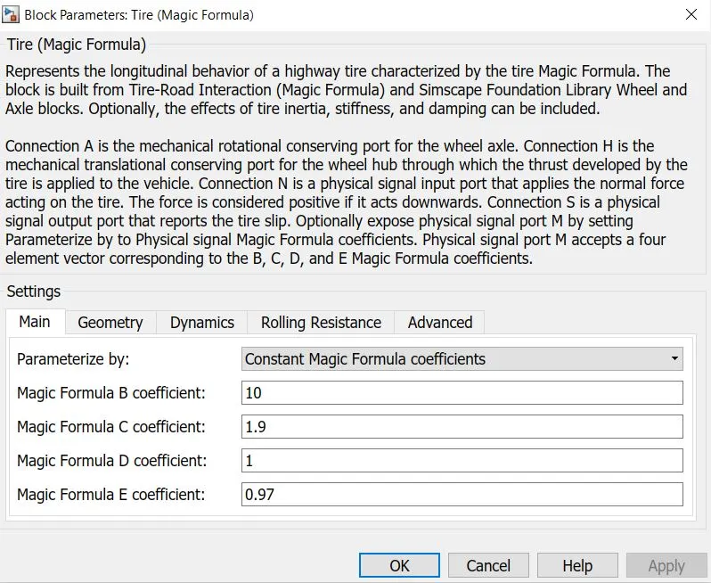
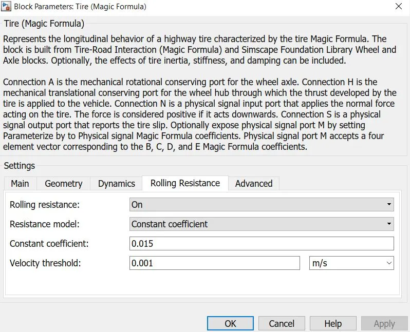
Tire (Magic formula) – this block represents a tire which is characterized by magic formula coefficients. It allows us to include effect of tire inertia, stiffness and damping. It has four connection, in which A is reserve for axel or mechanical rotational reserve port, connection H is for Hub, connection N takes normal force and connection S takes slip. Tire is parameterized by constant magic formula coefficients and rolling radius is 0.5m and coefficient of rolling resistance is 0.303.

Inertia – it represents ideal inertia. We gave value of inertia 100 Kg*m^2 .

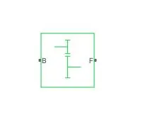
Simple gear – it represents a gear box with fixed- gear ratio. Connection B and F are mechanical rotation converting port. We used gear ratio 9.

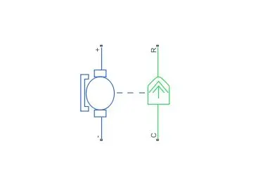
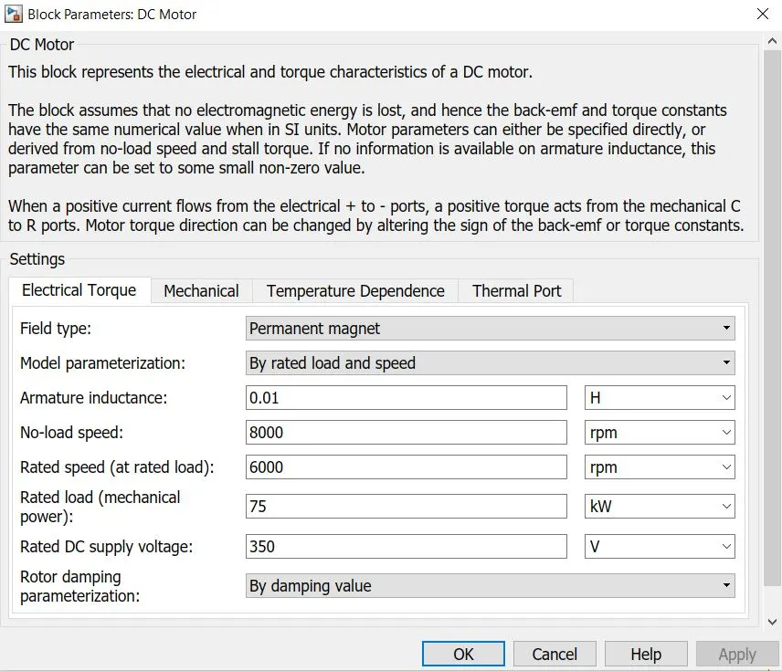
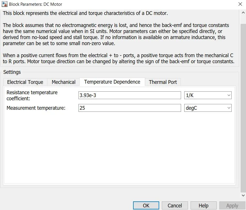
DC Motor -this block represents the electrical and torque characteristics of a DC motor. We used permanent magnet type DC motor with some default parameters. It is taking 330V and it is parameterized by equal circuit parameters. We used thermal parameter of motor to find temperature rise of motor.

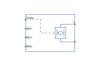
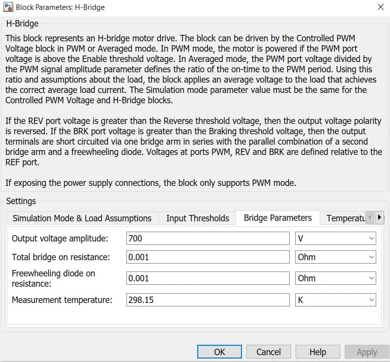
H-bridge – it represents an H-bridge motor drive. This block can be driven by PWM voltage in PWM or averaged mode, but PWM mode takes much time to complete simulation, so we are using averaged mode. Power supply is internal, and it is giving 330V. H-bridge takes PWM, reference, reverse and break signal.

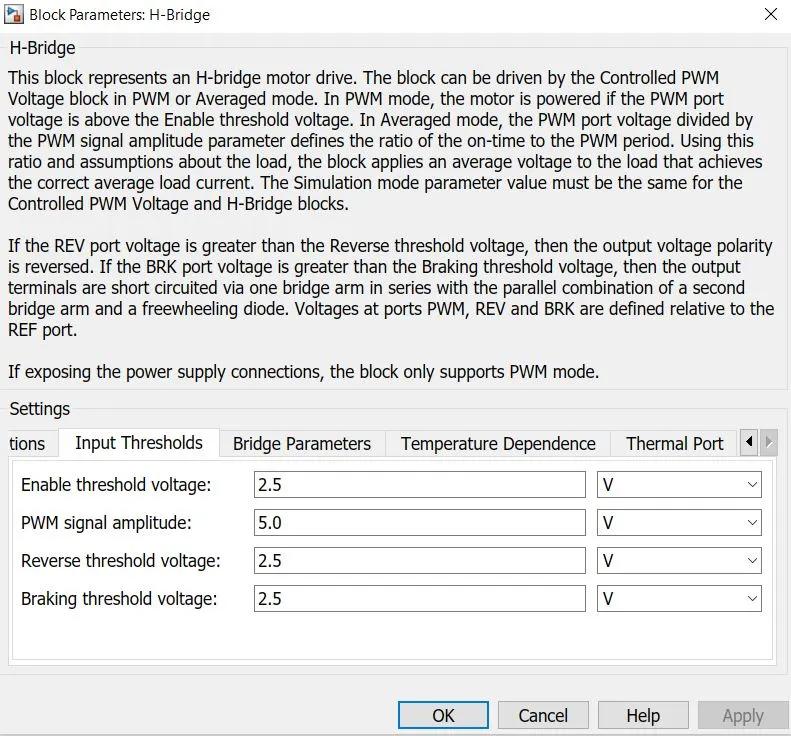
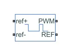
Controlled PWM voltage – this block creates PWM signal across reference and PWM port. The output voltage is zero when the pulse is zero and it is equal to output voltage, when pulse is high. We can choose simulation mode between PWM and averaged. We used averaged mode.

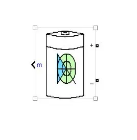
Battery – it implements a generic model for most popular battery types. Temperature and aging effect can be added. We used li-ion battery with nominal voltage 330V.

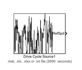
Drive cycle source – it generates a standard or user define longitudinal drive cycle. We can import drive cycle from workspace or from excel file.

Scope – it displays generated signal during simulation.

PS-Simulink – it converts physical signal into Simulink signal.

Simulink-PS – it converts Simulink signal to physical signal.

Display – it displays the value of signal.

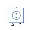
Controlled voltage source – it represents an ideal voltage source which maintains a specific voltage regardless of current.

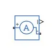
Current sensor – this block represents an ideal current sensor, which measures current in the circuit.

Gain – it multiplies a constant to a matrix.

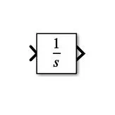
Integrator – it integrators input signal.

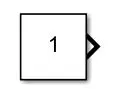
Constant – this block gives a constant value.

Sum – it adds or subtracts the input values.

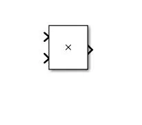
Product – it outputs the product of input values.

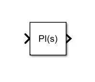
PI controller – this block implements continuous and discrete time PID control algorithm. We can choose controller type like – PID, PI, PD etc. PID values can be autotuned by its autotune feature.

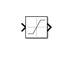
Saturation – this block limits input values to lower and upper saturation values.

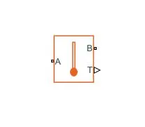
Temperature sensor – this block represents an ideal temperature sensor. Port A and port B connected to component and T port gives output.

Goto – Send signal to from port, with a specified tag.

From – takes signal from Goto block.

Bus creator – this block creates a bus signal.

Result –

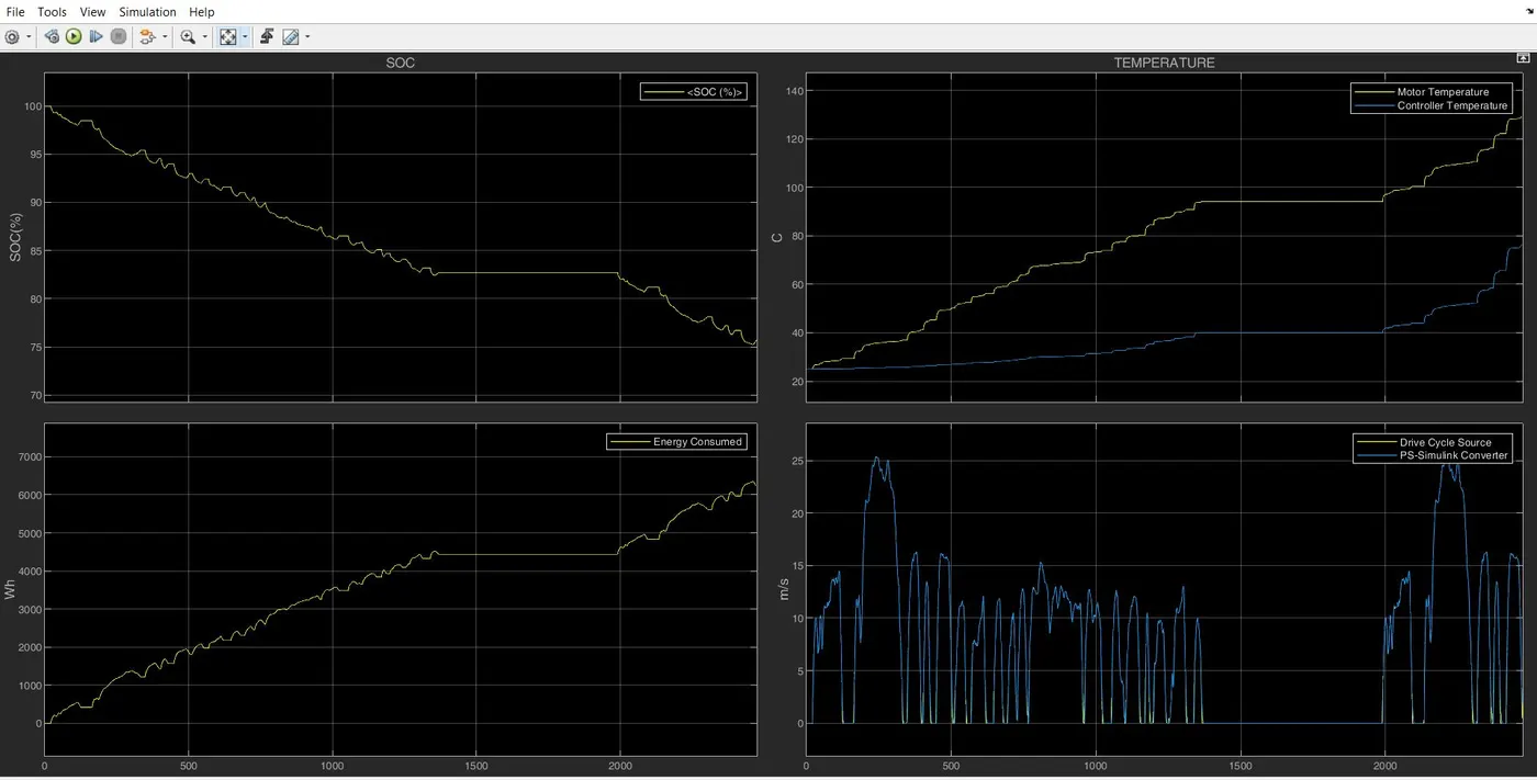
1. Drive Cycle – FTP75(2474s)
2. Energy consumed – 6.2KW
3. SOC(%) – 76
4. Temperature Rise – Motor -103°C, Controller – 50°C
5. Wind velocity(m/s) – 0

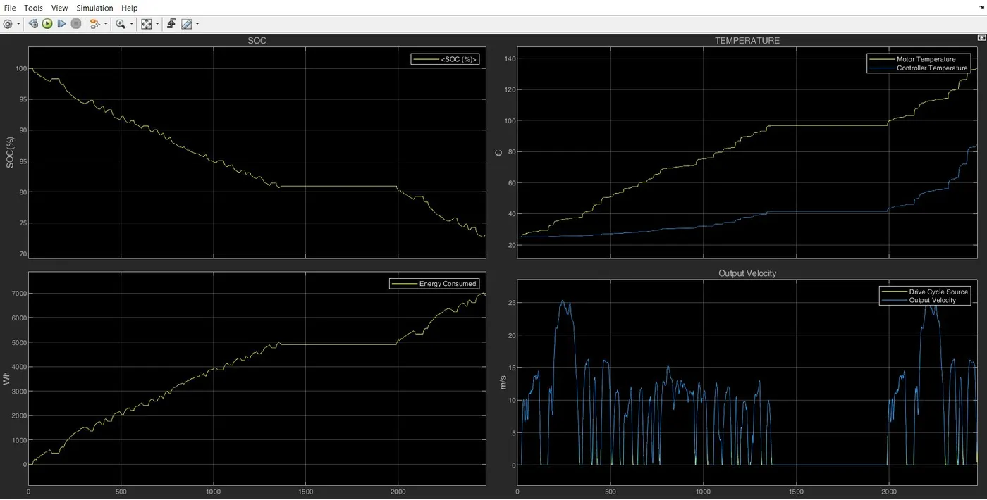
Now with same parameters and drive cycle, we simulated for wind velocity of 15Km/hr. According to theory energy consumption should be increased and that happened in simulation. Vehicle is consuming 693Wh more than normal condition. Motor temperature and controller temperature has also increased.

Conclusion –

We modelled electric vehicle model in Simulink, and it was successfully simulated. Output velocity is following reference velocity, so we can deduce, our model is working well. We successfully designed our driver block as well, which is providing acceleration and deacceleration signal.